

Journey through Various Regularization Techniques in Neural Networks
Course Lessons
| S.No | Lesson Title |
|---|---|
| 1 | Introduction |
| 2 | Overfitting in Neural Networks |
| 3 |
Why do we need Regularization? |
| 4 |
Types of Regularization Techniques |
| 4.1 | Number of Hidden layers and Hidden Neurons |
| 4.2 | Weight Decay |
| 4.3 | Batch Normalization |
| 4.4 | DropOut |
| 4.5 | Early Stopping |
| 4.6 | Data Augmentation |
| 5 | Conclusion |
Introduction
"Data is the new oil." - This is a very common phrase nowadays and you must have heard or read it somewhere. But why is it so? What problems does it create? Let us try to understand.
Almost all applications today include complex models such as neural networks, machine learning models, etc. But training complex models which can generalize better is a challenging problem. A model trained on a small dataset will fail to learn the problem, so we need large data and therefore "Data is the new oil" makes sense. But models trained on a large dataset give small training errors but large validation errors and consequently large test errors
Overfitting in Neural Networks
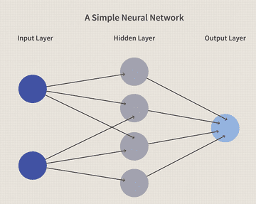
Before moving on to the overfitting problem, let us understand a basic neural network. Neural Networks consist of an input layer, hidden layer, and an output layer. These layers contain information in the form of neurons which are generally known as nodes. All the nodes in the adjacent layers are connected to each other.
Below I have attached an image of a simple neural network with 2 input neurons, 4 hidden neurons, and 1 output neuron. Here I will recommend you to read an article on neural networks to get a big picture of the neural network.
Neural Networks are successful because of the amount of data that we have. But with a large amount of data, there are high chances of noise which will result in high variance and consequently overfitting. As a result, our model will give accurate results on the training data but will fail on the validation and test data. Here is the illustration which is explained in detail below.
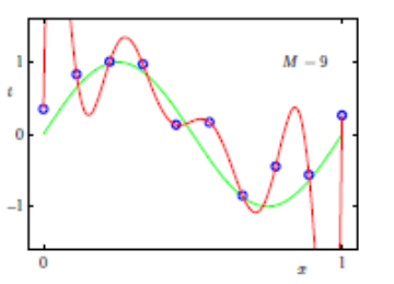
In the above picture, we want to learn a sinusoidal curve using the given sine values. But our model learns the red polynomial curve, which essentially gives low error on the blue training points but will fail on the validation and test points. As the dataset is large, I want you to point out the noise in the above illustration.
If you understood my point, the blue points which are not on the green sinusoidal curve are noise in our dataset. And this noise leads to high variance. We call this problem an Overfitting problem. The failure of neural networks on large data sets leads us towards regularization techniques.
Why do we need Regularization?
In the above picture, we want to learn a sinusoidal curve using the given sine values. But our model learns the red polynomial curve, which essentially gives low error on the blue training points but will fail on the validation and test points. As the dataset is large, I want you to point out the noise in the above illustration.
If you understood my point, the blue points which are not on the green sinusoidal curve are noise in our dataset. And this noise leads to high variance. We call this problem an Overfitting problem. The failure of neural networks on large data sets leads us towards regularization techniques.
Types of Regularization Techniques
With the introduction of neural networks, the next big problem was the generalization of neural networks. In this section, we will learn about different regularization techniques which are used for better generalization of neural networks.
Number of Hidden Layers and Hidden Neurons
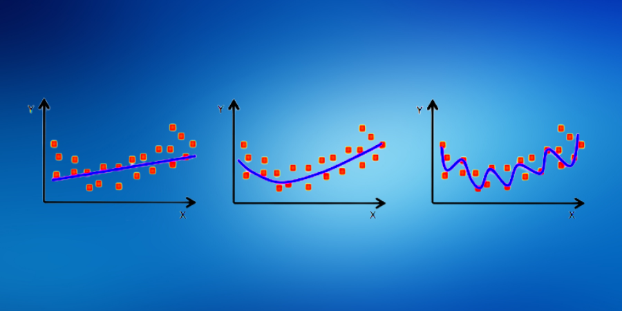
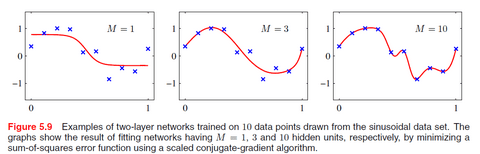
In a Neural Network, input and output nodes are determined by the dimensionality of the dataset. So, these nodes are fixed and cannot be changed. But the nodes in the hidden layers are free parameters and can be adjusted to give the best performance. So, consider a sinusoidal regression problem where the error is the mean squared error. In this regression problem, our aim is to try different numbers of hidden neurons and plot the output to see the best setting for our neuron. So, as you can see, when the numbers of hidden neurons are less, the curve is underfitting and as we increase the number of hidden neurons, the curve starts overfitting. The best setting is obtained at the number of hidden neurons to be equal to 8. So, careful initialization is important to prevent overfitting. We can plot such a graph to see if our model is overfitting.
Weight Decay
Another method of regularization is to start with a large number of hidden neurons and add a regularization term in the loss function. The regularization terms can be L2 regularization or L1 regularization.
Error function with L2 Regularization
E(w)‐‐ = E(w) + λ/2(WTW)
Error function with L1 Regularization
E(w)‐‐ = E(w) + λ ∥w∥
The effective model complexity is now determined by the choice of regularization coefficient lambda(λ). L1 Regularization brings sparsity to our model. For example, if we are predicting house prices from a number of features. It is highly likely that some of those features do not affect our house price prediction and some of the features may be highly correlated. L1 regularization pushes their weights towards 0 so that they do not affect our model predictions. While L2 Regularization results in non-sparse solutions. The features whose weights are pushed towards zero by L1 Regularization may have some effect on the house price prediction. So L2 Regularization pushes weights to be small rather than zero.
Batch Normalization
We divide our data into mini-batches and then pass it into the neural network.
With a slight change in the distribution of mini-batch input, it will result in large and larger changes in the successive layers. When the network is deeper, then the change in the deeper layers will also be very large. Since the small change gets multiplied by various weights as well as is passed through the activation functions multiple times. So with a small change in two batches, the successive layers will see these batches to be very different. A layer in the neural network may see these batches with very different distributions. This problem is also known as internal covariate shift. The batches have different mean and different variance. So we use batch normalization to solve this problem. Whenever it gets a batch of input, it will normalize that batch first into a normal distribution with 0 mean and variance 1 and then scale it to a factor of gamma and shift by beta. So the distribution now has a mean and variance. Gamma and beta are learned by backpropagation. In doing so, a little noise is also added in the inputs, and batch normalization can also act as a regulariser to prevent overfitting but the noise added is so small that we cannot use it as a complete regulariser. The above normalization results in the same distribution for all batches after a particular layer and helps to have faster convergence. Since the inputs to a particular layer are coming from the same distribution, it increases the learning rate.
DropOut
Ensemble methods nearly always improve the accuracy in machine learning models. If we want to use ensembles in neural networks, we will have to train different neural network architecture and then take the average of all these trained architectures. But training different neural network architectures will be very computationally expensive.
Dropout is a technique that addresses this issue. It prevents overfitting and provides a way of combining different neural networks efficiently. It randomly drops nodes temporarily along with all its incoming and outgoing connections in the adjacent layers. We assign a probability(p) of retaining modes where p is basically found using a validation set or simply set to 0.5. So, Every epoch of the neural network has a different architecture based on the nodes which will be retained. During testing, all the nodes are used and their weights are multiplied with the probability p.
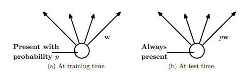
The above image explains the difference between training and testing. It largely reduces overfitting and gives better accuracy as compared to architectures without dropout.
Early Stopping
Training and Validation Loss in Neural Networks starts decreasing after each epoch but after a certain epoch, we will notice that the validation loss is no longer reducing. It may remain constant or may start increasing. So, by early Stopping, we observe the epoch where our validation loss reaches minima and then starts to increase or remains constant. We will train our network up to the observed epoch and this results in better results and avoids overfitting.
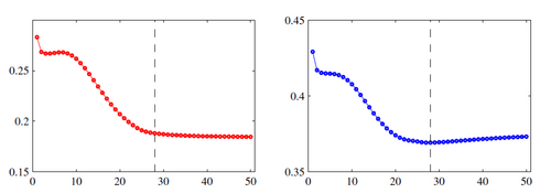
The above picture shows the training loss on the left and the validation loss on the right. So as we can see, validation loss is minimum on the dashed line, we will stop training our network at this point.
Data Augmentation
Data Augmentation can also be used as a regularization technique where we have a small amount of data. Data Augmentation includes various techniques such as Cropping, Flipping, Shearing, Zoom in/Zoom Out, Rotation, etc.
Conclusion
That's all from my side on different Regularization techniques which are used in complex models such as neural networks. You will be using almost all these techniques in your project based on neural networks.
References
- Chapter 5, Section 5.5 of Bishop - Pattern Recognition and Machine Learning