Introduction to Quantum Computing for Machine Learning

S.No	Lesson Title
1	Introduction
2	Basics of Quantum Computing
2.1	Bra-Ket Notation
2.2	Superposition
2.3	Entanglement
2.4	The Bloch Sphere
2.5	Quantum Decoherence
3	Quantum Machine Learning(QML) with Algorithms
3.1	QML to Solve Linear Algebra Problems
3.2	Quantum Principal Component Analysis
3.3	Quantum Support Vector Machines
3.4	Quantum Deep Learning
4	Conclusion
5	References

Introduction

As an outcome of decades of hard work quantum computing has finally found its way with the advancement of technology to realize quantum computers. There has been interest from many big firms like IBM, Microsoft, Google, etc. as they know about the serious number-crunching abilities of quantum computers. Until a few years ago quantum computers were only in theory until serious breakthroughs were made in the field of hardware required to make these machines a reality. It is often considered that the famous physicist Richard Feynman was one of the earliest conceptualizers of the theory of quantum computers. The idea of quantum computers is important to model the vast intricacies of nature as nature is built on top of quantum mechanics which cannot be modeled by classical computing techniques we use.

One of the most important properties of quantum computers is their ability to crunch numbers at a really high rate. For example, take a book in a library and mark an X on one of its pages. Now keep this book among 1 million other books in the library. Now you use a classical computer using 1 and 0 bits as well as a quantum computer using qubits to find that page. It'll take moments for the quantum computer to find that page whereas the classical computer will have to go through all the pages to find that X. This happens because of the interesting properties of quantum mechanics that we'll discuss in this article. We'll also discuss how quantum learning techniques have been applied to machine learning to give birth to a whole new field called quantum machine learning. Let's get started!

Basics of Quantum Computing

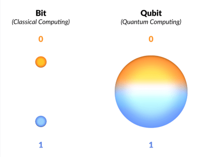
The major difference between quantum computers and traditional computers is that the traditional computer works on bits of data that are binary, or Boolean, with only two possible values: 0 or 1. On the other hand, quantum computers use something called "qubits". Qubits act like atoms in quantum computers. There are many tools in quantum physics that describe the interaction between different atoms. An atom can act as both particle and wave with the waveform having the capability of storing enormous amounts of data compared to a particle (or bit).

A quantum computer uses these qubits to supply information and communicate. The most important property of qubits is that they are encoded with quantum information in both states 0 and 1 instead of classical bits which can only take values 0 or 1. This means a qubit can be in multiple places at the same time due to superposition and hold an enormous amount of data. have a look at the following figure to understand how qubits can be distributed.

If all the things discussed above went above your head then don't worry. Now we'll discuss some basics of quantum computing and then we'll get back to more high-level concepts.

Bra-Ket Notation

This is a commonly used notation to write equations in quantum mechanics and quantum physics. This is a must-know for everyone because it's commonly used in research papers and blogs related to quantum computing.

The notation uses angle brackets < > and vertical bar | to construct "bras" and "kets". A "ket" looks like this : |v>. It denotes a vector mathematically, in a complex space v. In physical terms it represents the state of a quantum system.

A bra looks like: <f| . In mathematical terms, it denotes a linear function f: V → C which maps each vector in V to a number in complex plane C. A linear function acting on a vector is written as (<f| act on a vector |V>):

<f|v> ⍷ C

Wave functions and other quantum states can be represented in the complex vector space using the Bra-ket notation.

Superposition

Now let's revisit the concept of "qubits". You know that that quantum computer uses them instead of using the standard bits which take only two values i.e. 0 and 1. For a formal definition, qubit stands for quantum binary digit. Qubits can have multiple states at the same time with the value ranging between 0 and 1. Take the example of a coin toss with heads being 0 and tails being 1. When you toss the coin you don't know what will be the outcome until the coin lands. In other words, the outcome will exist in two different states simultaneously. This is the idea of superposition which is one of the core characteristics of quantum mechanics.

Superposition states that Qubits can exist in a combination of two states simultaneously. Another analogy to explain superposition can be when a high and low note from a musical instrument is played at the same time. This sound is neither high nor low note but a combination of two. But there's a catch - in a system following quantum mechanics you cannot directly observe superposition. If you try to measure a state of superposition that was indeterminate till a point becomes determinate as soon as you measure it. This gives a false idea that there is no superposition because you have already managed to determine a state of superposition separately.

Entanglement

Another fundamental principle of quantum mechanics is entanglement. To understand this we'll take another analogy of a game of wishbone. In this game, you both pull on one side of the wishbone to break it into two pieces but never look at each other's pieces to compare which one is bigger. Now in a quantum sense, as soon as you and your friend have your pieces, two things are possible: you have the biggest piece and your friend has the smaller one or vice-versa. You can also think of it as the wishbone pieces that have not yet decided which one is smaller or which one is bigger. Each wishbone piece is in superposition and their states are indeterminate. Now you need to go far away from each other and see which piece you have. As soon as you see your piece is larger it immediately determines the state of the piece your friend has.

Both the pieces were entangled but as soon as you see which piece you have your friends' piece is compelled into becoming the complementary piece. In other words, as soon as you decide to see which piece is yours the other piece loses its superposition. In a similar fashion, qubits are considered entangled if you can't describe the state of one qubit without describing the state of another- their states cannot be separated.

The Bloch Sphere

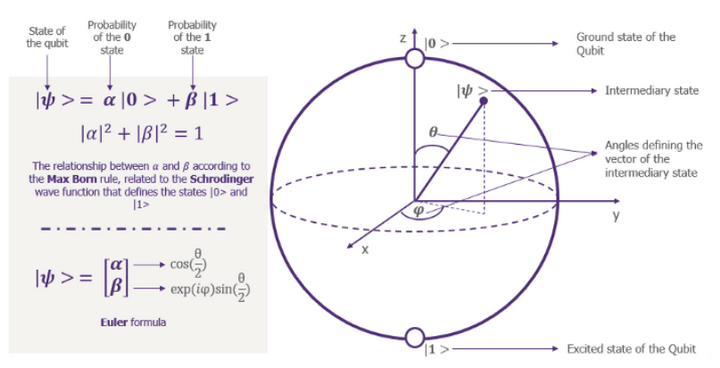
Now let's talk about The Bloch Sphere which is the mathematical representation of a qubit. It uses a two-dimensional vector with a normal length of one to represent the state of a qubit. There are two elements of this vector: a real number α and a complex number β. Have a look at the following figure and the equations mentioned to have a clearer idea of how the state of a qubit is represented:

Quantum Decoherence

Another important phenomenon is quantum decoherence. This happens when qubits superimpose and unwanted collapses happen randomly and naturally because of the noise in the system. This leads to errors in computation. Take the case where we think a qubit is in a superposition when it isn't and we do an operation on it, we'll get a completely different answer in this scenario. Quantum decoherence is caused by the contact of quantum systems with the environment and this is the reason that they need to be separated from the environment. When qubits interact with the environment information leaks out from that and information from the environment leaks into them. The information that leaks out could have been important for some future calculations but the information that leaks in is random noise.

Quantum Coherence helps the quantum computer to process information in a way that classical computers cannot. A quantum algorithm performs a stepwise procedure to solve a problem, such as searching a database. It can outperform the best-known classical algorithms. This phenomenon is called the Quantum Speedup.

Quantum Machine Learning(QML) with Algorithms

Quantum computers use various methods that are derived from classical machine learning to solve problems pertaining to data science. Following are some of those techniques/algorithms:

Quantum Machine Learning to Solve Linear Algebra Problems

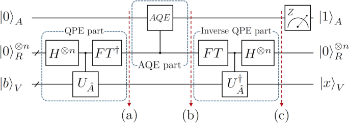
A wide range of machine learning algorithms consist of matrix operations in a high dimensional vector space. In quantum computing, the quantum state of the qubits is a vector in 2^d - dimensional complex vector space. A lot of matrix transformations happen in this space. Quantum Computers can solve common linear algebraic problems such as the Fourier Transformation, finding eigenvectors and eigenvalues, and solving linear sets of equations over 2^a- dimensional vector spaces in time that is polynomial in a (and exponentially faster than classical computers due to the Quantum Speedup). One of the examples is the Harrow, Hassidim, and Lloyd (HHL) algorithm. Following is the circuit diagram for the same algorithm:

Quantum Principal Component Analysis

Principal Component Analysis (PCA) is used for dimensionality reduction and is one of the most popular algorithms in the field of classical machine learning. Dimensionality reduction comes at the cost of accuracy but if done correctly it makes the machine learning task much more comfortable because it's convenient to deal with a smaller dataset.

Take the dataset which has only 10 attributes, now it'll be easier to apply PCA to this dataset and get really good results. But when we have millions of attributes it becomes difficult to apply PCA because the importance of one attribute when compared to another in quantifying the overall variance of the dataset is very difficult to predict.

Another issue with classical techniques is that they are not good at calculating eigenvectors and eigenvalues when the dimensions of the dataset are very large. Quantum computers solve this issue by using Quantum Random Access Memory (QRAM) to choose a data vector at random. It maps that vector into a quantum state using qubits. The summarized vector that we get after Quantum Principal Component Analysis has logarithmic qubits. The chosen random vector forms a dense matrix. This matrix is called the covariance matrix.

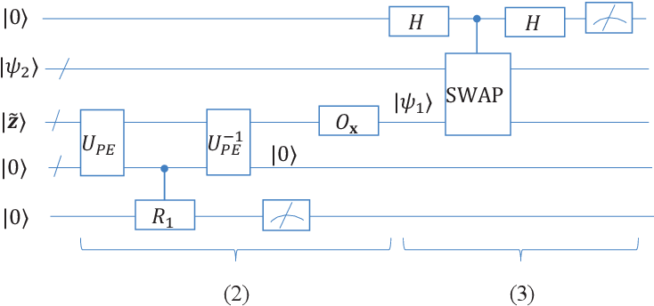
By repeatedly sampling the data and using a trick called density matrix exponentiation, combined with the quantum phase estimation algorithm (which calculates the eigenvectors and eigenvalues of the matrices), we can take the quantum version of any data vector and decompose it into its principal components. Both the computational complexity and time complexity are thus reduced exponentially. Following is a diagram of the quantum circuit to perform Principal Component Analysis:

Quantum Support Vector Machines

Support Vector Machine is a classical machine learning algorithm. It classifies the linearly separable data into two different classes but if the data is not linearly separable then it's superimposed to a higher dimension and the dimensionality keeps on increasing until the data becomes linearly separable.

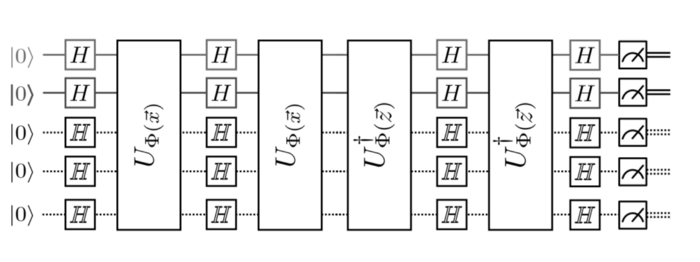
There's an issue with continuously increasing the dimensionality of the data when it comes to classical computers as after a particular limit these computers don't have enough processing power to process high dimensional data. This is where quantum computing comes in. Quantum computers can perform calculations for support vector machines at an exponentially faster rate using the principles of superposition and entanglement. Following is a diagram for the quantum circuit to perform SVM:

Quantum Deep Learning

Quantum computing can be combined with deep learning to reduce the time required to train a neural network. As you know, when the size of a neural network increases the time and the computational power required to train it increases. The solution to this is to mimic classic deep learning algorithms on an actual quantum computer.

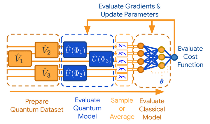
Quantum computers are designed in such a way that the hardware can mimic a neural network instead of the software used in classical computers. Here, a qubit acts as a neuron that constitutes the basic unit of a neural network. Thus quantum computers that have a sufficient number of qubits can be used for deep learning with performance that easily surpasses that of a deep learning model on a classical computer. Following is an example of how a deep learning network using quantum computers will look like:

Conclusion

In this article, we covered different aspects of quantum computing starting from basics to how it can be used for machine learning. Quantum computing is a growing field with many more discoveries to be made. The rise of quantum computing will surely change the landscape of machine learning and how the algorithms are implemented using classical computing techniques. Happy learning!

References

1. https://ai.googleblog.com/2021/06/quantum-machine-learning-and-power-of.html
2. https://blog.paperspace.com/beginners-guide-to-quantum-machine-learning/