Recurrent Neural Networks

S.No	Lesson Title
1	Introduction
2	Applications of Recurrent Neural Networks
2.1	Sentiment Analysis
2.2	Image Captioning
3	What are Recurrent Neural Networks?
3.1	Understanding MLP
3.2	Understanding RNN
3.3	Understanding a Recurrent Neuron in Detail
4	Implementation
4.1	Importing and Preprocessing Dataset
4.2	Model Creation
4.3	Model Training
5	Conclusion

Introduction

There are many tasks in our daily life wherein the sequence of our data matters. For example, in a sentence, all the words need to follow a particular sequence. If the words are not in a sequence then the sentence will not have any meaning. Another example is time-series data, where the time defines whether an event occurs. There are many more cases where the sequence of the information has a significant role in determining the output. To solve such kinds of tasks, we need a network that can remember the prior data to give a reasonable output. This is where Recurrent Neural Networks come into play.

Applications of Recurrent Neural Networks

Sentiment Analysis

This can be a task of classifying tweet or movie reviews into positive or negative sentiment. Consider the example given below, here in our input, we would be having a tweet that would be of varying length and our model would need to understand the entire sentence in order to accurately classify that sentence.

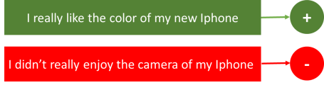
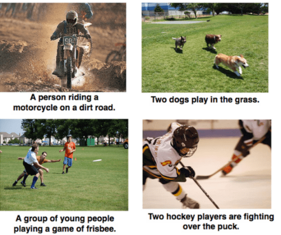
Image Captioning

Image captioning is a process of generating descriptive text summarizing the content present in the image. Here, the input will be an image and the output would be a sentence of varying lengths. Have a look at the examples shown below.

So we can use Recurrent Neural Networks to map inputs to outputs having different types and lengths. Now that we have seen some of their applications, let us understand more about recurrent neural networks.

What are Recurrent Neural Networks?

Understanding MLP

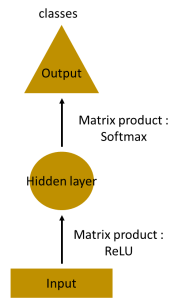
Let us say that we need to create a model which will predict the next word in a sentence. Let us understand what would happen if we used a Multi-Layered Perceptron to accomplish this task. In an MLP we have an input layer, a hidden layer, and an output layer.

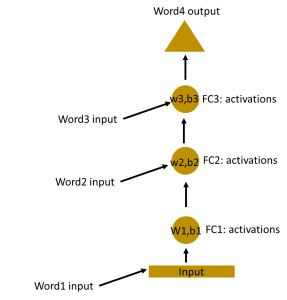
Let us see what will happen if we have a deeper network. In the below network, we can see that there are multiple hidden layers present. So here, the input layer receives, the input, then in the first hidden layer, activations are applied and then these activations are sent to the next hidden layer until the output is produced. As every hidden layer has its own weights, they act independently. Now if we need to detect relationships between successive inputs then we would need to apply inputs to the hidden layers.

Understanding RNN

In the above figure, all the weights and biases of the hidden layers are completely different. If we need to combine these hidden layers together then we would need to combine these weights and biases together. This is done in the figure below.

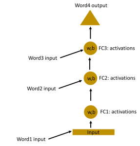
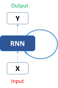
Now that we have made all the weights and biases of the hidden layers equal, we can roll the hidden layers in a single recurrent layer.

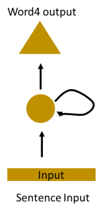
So a recurrent neural network stores the state of the previous input and combines it with the current input, hence some relationship between the current and previous input is preserved.

Understanding a Recurrent Neuron in Detail

Let us get a better understanding of the recurrent neural network by performing a simple task. Let us take the word "Hello". We will provide the RNN model with the first 4 letters which are h,e,l,l, and the RNN will predict the last letter which is 'o'. In this case our vocabulary is just {h,e,l,o}.

Let us see how RNN will predict the fifth letter that is 'o'. In the above figure, we can see that the blue RNN block uses a recurrence formula to the input vector and also to its previous state. In our sample case, the first letter is 'h' and it has nothing before it, so let's move on to the next letter which is 'e'. In this case, a recurrence formula is applied to the letter 'e' and to the previous letter which is 'h'. This is called a time step. So if at time t, the input is 'e' and at time t-1, the input is 'h', then the recurrence formula will be applied to both 'e' and 'h'. The formula for the current state is as follows:

h_t =f(h_t-1,x_t)

In the above formula h_t is the new state, h_t-1 is the previous state and x_t is the current input. Now we have a state of the previous input instead of the input itself. This is because the input neuron would have applied the transformations on the previous input. In our sample case, we only have 4 inputs that we need to feed to the network. So, during the recurrence formula, the same function and the same weights are applied to the network at each time step. Let us assume that the activation function is tanh, the weight of the RNN cell is W_hh and the weight of the input neuron is W_xh. From this, we can see the recurrence relation below.

h_t =tanh(W_hhh_t-1+W_xhx_t)

The RNN cell in this case is just taking the immediately previous state into consideration. When the final state is calculated the output can be produced.

The output can be calculated by the below formula:

y_t = W_hyh_t

Implementation

In this project, we will be making a sentiment classifier for the IMDB movie reviews dataset. We would be using the IMDB dataset from keras library.

Importing and Preprocessing Dataset

Firstly let us import the dataset

#Here we are importing the imdb reviews dataset from keras

from keras.datasets import imdb
((XT,YT),(Xt,Yt)) = imdb.load_data(num_words=10000)

We have now imported the IMDB review dataset from keras. We have taken the number of unique words in our dataset to be 10000 and we have stored this dataset into 4 variables. XT, YT contains the training data, and Xt, Yt contains the testing data. We will now explore this dataset a bit before creating our model.

#Here we are seeing the first sentence in our dataset
print(XT[0])
print(YT[0])
print(len(XT))
print(len(Xt))
print(XT.shape)

Output:

[1, 14, 22, 16, 43, 530, 973, 1622, 1385, 65, 458, 4468, 66, 3941, 4, 173, 36, 256, 5, 25, 100, 43, 838, 112, 50, 670, 2, 9, 35, 480, 
284, 5, 150, 4, 172, 112, 167, 2, 336, 385, 39, 4, 172, 4536, 1111, 17, 546, 38, 13, 447, 4, 192, 50, 16, 6, 147, 2025, 19, 14, 22, 4, 
1920, 4613, 469, 4, 22, 71, 87, 12, 16, 43, 530, 38, 76, 15, 13, 1247, 4, 22, 17, 515, 17, 12, 16, 626, 18, 2, 5, 62, 386, 12, 8, 316, 8, 
106, 5, 4, 2223, 5244, 16, 480, 66, 3785, 33, 4, 130, 12, 16, 38, 619, 5, 25, 124, 51, 36, 135, 48, 25, 1415, 33, 6, 22, 12, 215, 28, 77, 
52, 5, 14, 407, 16, 82, 2, 8, 4, 107, 117, 5952, 15, 256, 4, 2, 7, 3766, 5, 723, 36, 71, 43, 530, 476, 26, 400, 317, 46, 7, 4, 2, 1029, 13, 
104, 88, 4, 381, 15, 297, 98, 32, 2071, 56, 26, 141, 6, 194, 7486, 18, 4, 226, 22, 21, 134, 476, 26, 480, 5, 144, 30, 5535, 18, 51, 36, 
28, 224, 92, 25, 104, 4, 226, 65, 16, 38, 1334, 88, 12, 16, 283, 5, 16, 4472, 113, 103, 32, 15, 16, 5345, 19, 178, 32]
1
25000
25000
(25000,)

We can see that the dataset is already preprocessed. All the words in the sentences are replaced by their appropriate indices in the vocabulary. We have 25000 sentences in the training data and 25000 sentences in the testing data. We can see that the shape of the training data is (25000,). This means that the sentences are not of equal length. We would need to make the sentences of equal length before training our model on this data.

Before that let us see what is the first sentence.

#Here we are getting the word_index dictionary for this dataset and printing the first sentence in our dataset.
word_idx = imdb.get_word_index()
idx_word = dict([value,key] for (key,value) in word_idx.items())
actual_review = ' '.join([idx_word.get(idx-3,'?') for idx in XT[0]])
print(actual_review)
print(len(actual_review.split()))

Output:

? this film was just brilliant casting location scenery story direction everyone's really suited the part they played and you could just imagine being there robert ? is an amazing actor and now the same being director ? father came from the same scottish island as myself so i loved the fact there was a real connection with this film the witty remarks throughout the film were great it was just brilliant so much that i bought the film as soon as it was released for ? and would recommend it to everyone to watch and the fly fishing was amazing really cried at the end it was so sad and you know what they say if you cry at a film it must have been good and this definitely was also ? to the two little boy's that played the ? of norman and paul they were just brilliant children are often left out of the ? list i think because the stars that play them all grown up are such a big profile for the whole film but these children are amazing and should be praised for what they have done don't you think the whole story was so lovely because it was true and was someone's life after all that was shared with us all
218

Here we are getting the word_index keras. This is a dictionary that maps each word to its index. In order to see the first sentence of the dataset, we need a dictionary that maps the index to a word. So, using word_idx, we created a variable idx_word, which maps the index to its corresponding word. After that, we are running a loop on the first sentence which is XT[0] and we are getting the words for every index and storing it in a variable named actual_review.

Now that we have visualized the first sentence, let us make every sentence of equal length. For this, we will use the pad_sequences function in keras.

#Here we are making each sentence of equal length using pad_sequences.
from keras.preprocessing import sequence

X_train = sequence.pad_sequences(XT,maxlen=500)
X_test = sequence.pad_sequences(Xt,maxlen=500)
print(X_train.shape)
print(X_test.shape)

Output:

(25000,500)
(25000,500)

We are giving each sentence a length of 500. This means that the sentences with a length greater than 500, will be cut to 500 and the sentences with a length less than 500 will get 0 inserted until their length becomes 500.

Model Creation

Now let us create our model.

#Here we are creating the creating our model architecture.
from keras.layers import Embedding,SimpleRNN,Dense
from keras.models import Sequential

model = Sequential()
model.add(Embedding(10000,64))
model.add(SimpleRNN(32))
model.add(Dense(1,activation='sigmoid'))
model.summary()

Output:

Model: "sequential"
_________________________________________________________________
Layer (type)                 Output Shape              Param #   
=================================================================
embedding (Embedding)        (None, None, 64)          640000    
_________________________________________________________________
simple_rnn (SimpleRNN)       (None, 32)                3104      
_________________________________________________________________
dense (Dense)                (None, 1)                 33        
=================================================================
Total params: 643,137
Trainable params: 643,137
Non-trainable params: 0
_________________________________________________________________

Our model is now created.

The embedding layer will create word embeddings for every single word in our dataset. We have kept the shape of this layer as (10000,64). This is because there are 10000 words in our dictionary and we are representing each word using 64 numbers. Initially, the embedding layer is randomly initialized, but as the model is trained, the embedding layer also gets trained.

In the RNN layer, we have 32 RNN cells. We can keep this any number we want.

Model Training

Now let us train our model and evaluate it.

#Here we are training our model.
model.compile(optimizer='rmsprop',loss='binary_crossentropy',metrics=['acc'])
hist = model.fit(X_train,YT,validation_split=0.2,epochs=5,batch_size=128)
model.evaluate(X_test,Yt)[1]

Output:

0.8325200080871582

Here we are training our model using the 'rmsprop' optimizer and we are evaluating it using the test dataset. We can see that our model achieved an accuracy of 83.25%.

Conclusion

In this article, we have explored the sequential data and how the recurrent neural network is exploited to model a neural network for handling the sequential data. We have also seen the wide range of applications of recurrent neural networks. Further, we have implemented a simple model to perform sentiment analysis on the IMDB dataset by using the keras library.