

Convolutional Neural Networks
Course Lessons
| S.No | Lesson Title |
|---|---|
| 1 | Introduction |
| 2 | Limitations of Basic Neural Network |
| 3 | Building blocks of CNN |
| 3.1 | Input Layer |
| 3.2 | Convolutional Layer |
| 3.3 | Pooling Layer |
| 3.4 | Fully Connected Layer |
| 3.5 | Softmax Layer |
| 4 |
Implementation |
| 4.1 | Importing Dataset |
| 4.2 | Preprocess Dataset |
| 4.3 | Model Creation |
| 4.4 | Model Training |
| 5 | Conclusion |
Introduction
Computer vision is a rapidly evolving domain with a plethora of methods and algorithms published on a daily basis. We all know that CNN or Convolutional Neural Networks is the driving force behind this shift. CNNs are extensively used in most computer vision tasks such as image classification, object detection, image segmentation, etc. In this report, we will delineate the limitations of the base neural network and the way CNN addresses it to deal with the challenging problems.
Limitations of Basic Neural Network
Let us illustrate the limitations of the traditional neural network with an example. Consider the MNIST dataset, we know that each image in MNIST dataset is of the shape 28 x 28 x 1. This means that it is a grayscale image and it has only one channel. So, if we are using a simple neural network then the total number of neurons in the input layer will be 28 x 28, which is 784. This number is still manageable. Now, if we have images of shape 100 x 100, then the number of neurons will increase by a great magnitude. CNN solves these problems. CNN helps to extract the features of an image and converts them into fewer dimensions.
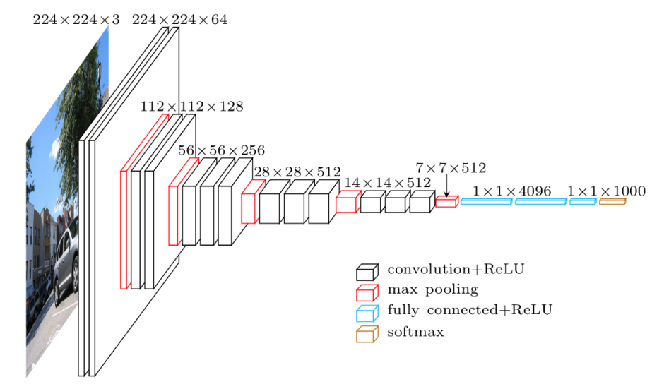
In the above figure, we can observe that we have an image of the shape of 224 x 224 x 3. This means that the image has 3 channels which are red (R), green (G), and blue (B) respectively. We are passing this image to many convolutional layers and finally, we are predicting the class of an image using softmax activation.
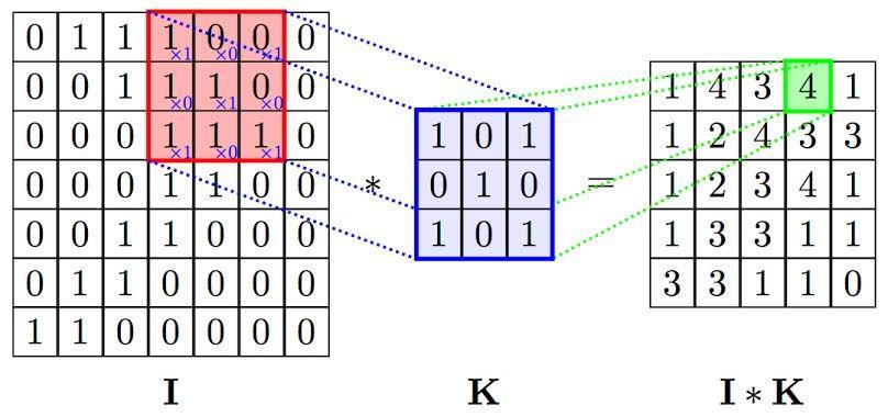
Now let us understand the convolutional operation. The matrix I is an image matrix of dimension 7 x 7. The matrix K is a filter matrix of dimension 3 x 3. The matrix K is placed on the matrix I (receptive field), and the kernel is convolved over the image matrix 'I' by multiplying the corresponding elements resulting in the matrix I*K.
With this kind of computation, we can find a particular feature from our image and we can produce convoluted features which will emphasize on the distinct features. The more filters we deploy, the more features CNN will extract.
Building blocks of CNN
Below is a list of the layers that we generally have in a CNN architecture.
- Input layer
- Convolutional layer
- Pooling layer
- Fully connected layer
- Output layer
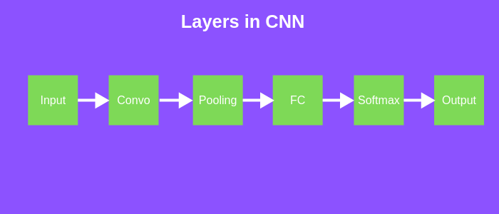
Different Layers of CNN
Input Layer
The input layer of a CNN architecture constitutes the image data. As we have observed in the previous example, the image data is represented by a 3D matrix. Let us say if have an image of shape 28 x 28, then we would need to convert it to 784 x 1 (1D vector) before we feed it to the input.
Convolutional Layer
The input layer of a CNN architecture will constitute the image data. As we have seen in the previous example, image data is represented by a 3D matrix. In the case of MNIST, we have input data of dimension 28x28x1 and such 60,000 images are used for the training phase and 10000 images are used for testing. Convolution operation many advantages such as 1) Sparse connection 2) Spatial relationship among the pixel intensities and 3) Equivariance.
Pooling Layer
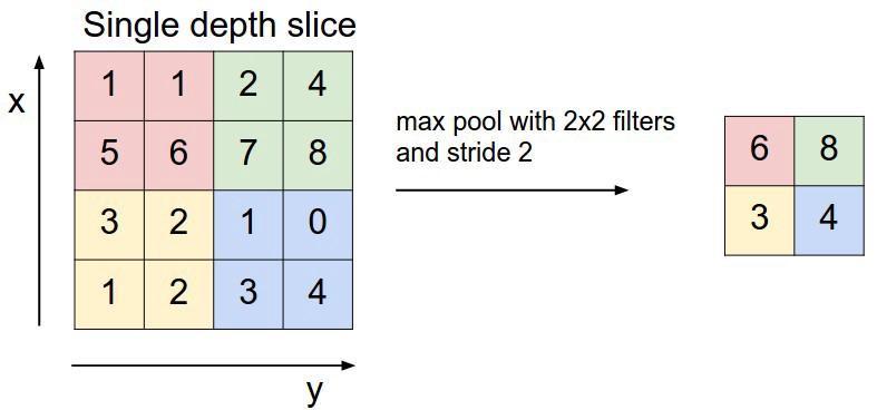
A pooling layer is used for reducing the spatial dimension in the convolutional neural network. If we use a fully connected layer after a convolutional layer then it will be computationally expensive. So we use a max-pooling layer, to reduce the size of the image. In the above example, we can see that a max-pooling operation has been performed with 2 x 2 filters and a stride of 2. Our input matrix is of the shape 4 x 4, and we use a filter of size 2 x 2 on it and we take the maximum element in the filter. After that, we take the next 2 x 2 matrix in our 4 x 4 matrix and repeat the same process.
In general, if we have input dimension W1 x H1 x D1, then
W2 = (W1-F)/S+1
H2 = (H1-F)/S+1
D2 = D1
where W2, H2 and D2 are the width, height and depth of output.
Fully Connected Layer
Fully connected layer is a dense layer (1D vector) . It has weights, biases and neurons. It connects the neurons in one layer to all the neurons in the other layer.
Softmax Layer
The softmax activation function is used in the classification layer. Softmax will give the probability distribution of the presence of a particular class. The neuron or the class with the highest probability maps the presence of that particular element or the object in the image.
Now that we have understood what a CNN is, we will see its implementation in keras.
Implementation
We will be creating a CNN architecture which can classify handwritten digits using the MNIST dataset. Let us first import all the libraries we need for our project.
Importing Dataset
#Here we have imported all the libraries required for our analysis

import numpy as np
import pandas as pd
import matplotlib.pyplot as plt

from keras.datasets import mnist
from keras.utils import to_categorical
from keras.layers import *
from keras.models import Sequential
Now that we have imported all the libraries, let us import our MNIST dataset from keras.
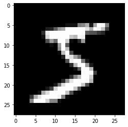
#Here we are importing and visualizing our MNIST data which we have imported from keras

(XTrain,YTrain),(XTest,YTest) = mnist.load_data()
plt.imshow(XTrain[0].reshape(28,28),cmap="gray")
Output:
Preprocess Dataset
As we can see, we have imported the MNIST dataset from keras and stored its variables (XTrain,YTrain),(XTest,YTest). We have also visualized our first image. Our next task is to pre-process our dataset.
#Here have created a function called preprocess_data,
#which will reshape our image to 28 x 28 x 1 and it will divide each element
#by 255.0 to rescale or normalize the image. After that we have passed
#our training and test dataset through this function.

def preprocess_data(X,Y):
    X = X.reshape((-1,28,28,1))
    X = X/255.0
    Y = to_categorical(Y)
    return X,Y

XTrain,YTrain = preprocess_data(XTrain,YTrain)

XTest,YTest = preprocess_data(XTest,YTest)
Now that we have pre processed our dataset, our next task is to create our CNN architecture.
Model Creation
#Here we are creating our CNN architecture

model = Sequential()
model.add(Conv2D(32,(3,3),activation='relu',input_shape=(28,28,1)))
model.add(MaxPool2D((2,2)))
model.add(Conv2D(64,(3,3),activation='relu')
model.add(MaxPool2D((2,2)))
model.add(Conv2D(64,(3,3),activation='relu')
model.add(Flatten())
model.add(Dense(64,activation='relu'))
model.add(Dense(10,activation='softmax'))

model.summary()
Output:
Model: "sequential_1"
_________________________________________________________________
Layer (type)                 Output Shape              Param #
=================================================================
conv2d_1 (Conv2D)            (None, 26, 26, 32)        320
_________________________________________________________________
max_pooling2d_1 (MaxPooling2 (None, 13, 13, 32)        0
_________________________________________________________________
conv2d_2 (Conv2D)            (None, 11, 11, 64)        18496
_________________________________________________________________
max_pooling2d_2 (MaxPooling2 (None, 5, 5, 64)          0
_________________________________________________________________
conv2d_3 (Conv2D)            (None, 3, 3, 64)          36928
_________________________________________________________________
flatten_1 (Flatten)          (None, 576)               0
_________________________________________________________________
dense_1 (Dense)              (None, 64)                36928
_________________________________________________________________
dense_2 (Dense)              (None, 10)                650
=================================================================
Total params: 93,322
Trainable params: 93,322
Non-trainable params: 0
_________________________________________________________________
As we can see that we have created our architecture. In the first layer we have a convolutional layer with 32 filters of the shape 3 x 3 with relu activation. After passing the image through this layer the shape of the image becomes 26 x 26 x 32. After this we have passed the image through a max pooling layer which has reduced the dimensions of our image. In the last layer we have a Fully Connected layer which has a softmax activation and 10 neurons corresponding to 10 classes.
Model Training
Finally let us train our model and evaluate it.
#Here we are training our model using adam optimizer and loss as categorical cross entropy.

 model.compile(optimizer='adam',loss='categorical_crossentropy',metrics=['accuracy'])
hist = model.fit(XTrain,YTrain,epochs=20,validation_split=0.1,batch_size=128)
model.evaluate(XTest,YTest)
Output:
10000/10000 [==============================] - 2s 208us/step
[0.034403899156812225, 0.9921000003814697]
We have now trained our model for 20 epochs using adam optimizer. We can see that we are getting an accuracy of 99.21% on our test data.
Conclusion
In this article, we have discussed the driving force behind the challenging computer vision tasks. We have also discussed the various layers or the building block that constitutes the CNN. Further, we have demonstrated the implementation of CNN on the MNIST database. Happy Learning!