

Evolution of Design of Artificial Neuron
Course Lessons
| S.No | Lesson Title |
|---|---|
| 1 | Introduction |
| 2 | Biological Neuron |
| 3 | McCulloh Pitts (MCP) Neuron |
| 4 | Perceptron |
| 5 | Adaline |
| 6 | Madaline |
| 7 | Conclusion |
Introduction
How did it all begin? This thought would have crossed everyone's mind while studying various concepts related to Artificial Intelligence. Another interesting thought is about the usage of the word "Neural" for deep learning models such as Artificial Neural Networks, Recurrent neural network, etc. This can lead to a vague idea that the concepts of these models are borrowed from the functioning of the human brain. To summarize all these thoughts we'll take a deeper dive into the past to see how neural networks were born and how they progressed over time. Also, the parallelism that is drawn with biological neurons will be discussed briefly.
Biological Neuron
Before we talk about any preliminary models that mimic the biological neuron let's have a look at how biological neurons work. Following is a simplified representation of a neuron:
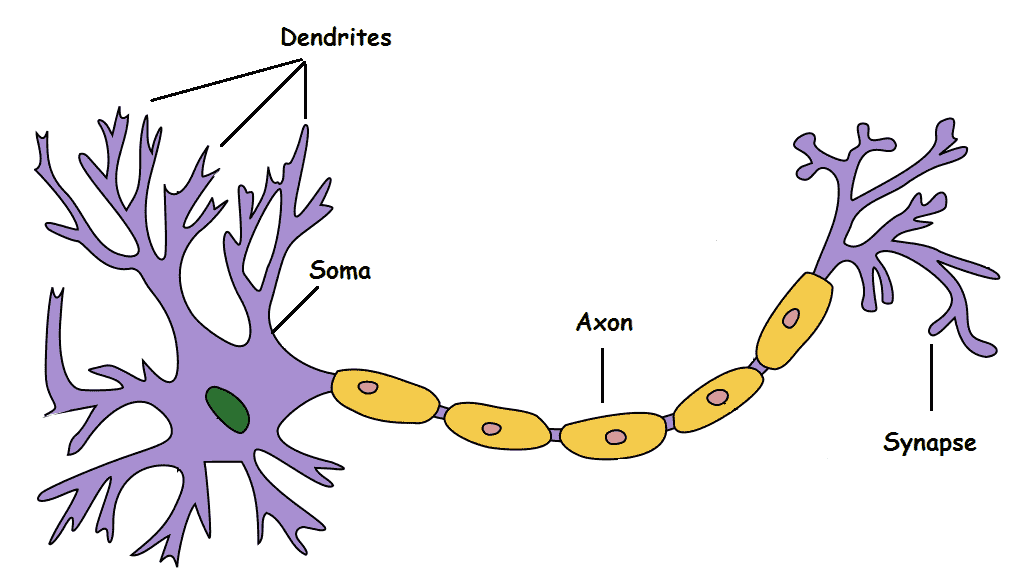
It has 4 different components:
- Dendrite - Takes the signal(input) from other neurons
- Soma - Processes the information in the signal
- Axon - Transmits the output from the neuron
- Synapse - Connects the neuron to other neurons to tranfer the processed signal
Let's have a look at how neurons work on a higher level. Dendrites take the input, the processing is done by Soma(CPU), the output is passed on to other neurons using a wire-like structure. To summarize it, neurons do the following things - take input, process the input, and then generate the output. Now in reality we have more than one neuron in our body and they make decisions based on the inputs they receive. For example, we are playing a sport like a football and there is a ball coming towards us then the signal from our eyes regarding that ball is passed down to our hands/feet through a network of neurons. But how many neurons do we have?
An estimate says that the human body has around 100 billion neurons, and they are inter-connected through complex networks with the smallest unit functioning close to what we showed above. Now in the flying ball example, not all the neurons are fired or activated at the same time. Only those neurons which can send signals to move our hand/feet to protect us from the ball are activated. This is an interesting property of biological neurons as they have a mechanism by which only relevant neurons are fired at a time. Another interesting property is that neurons are believed to have a hierarchical order and each layer of a neuron does a specific task.
With all this said about the biological neuron let's move on and talk about how artificial neurons were developed over the past few decades.
McCulloch Pitts(MCP) Neuron
The most fundamental unit of a deep neural network is an artificial neuron. The very first attempt at building an artificial neuron to mimic the functionality of a biological neuron was made by McCulloh (neuroscientist) and Pitts(logician) in 1943 in their research paper entitled "A Logical Calculus Of The Ideas Immanent In Nervous Activity". Following is a schematic representation of their proposed artificial neuron.
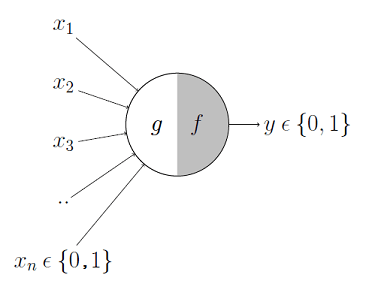
Now the functioning of this unit can be divided into two parts. Let's try to understand the functioning of these two units with an example where we say yes to eating an ice cream based on different inputs we get. Assume that the inputs are flavor(x1), color (x2), sugar content(x3). Assume all the inputs have only two possibilities represented by binary digits (0,1) and the output is also binary (0 for no, 1 for yes). The first part is the input part where function g takes the inputs and performs an aggregation function by adding these inputs. Next, a function f takes the aggregated values and makes a decision based on a threshold theta.
Now, you'll want to eat the ice cream when it has your favorite flavor or it has less sugar or the color is attractive. These factors are taken into account by aggregating all the inputs. If the final value after aggregation is sufficiently larger than a threshold then you would surely like to eat the ice cream. Sounds efficient enough right? But there's a major issue, there's no learning associated with this model. Threshold values are manually assigned and can be different for different people. This means that we cannot have a model which is generalizable. So what next!!?
After realizing that there was no learning involved, in such a model many researchers tried to add a learning component to the model based on the errors it made and this led to the birth of the perceptron model. Let's have a look at it.
Perceptron
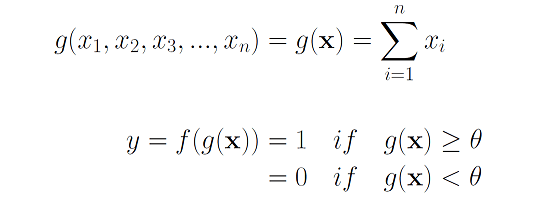
Perceptron was arguably the first model that had a self-training mechanism using which it could learn from the errors it made during prediction. It was introduced by Frank Rosenblatt in 1957 ("The perceptron: A probabilistic model for information storage and organization in the brain"). Following is a schematic representation of a single layer perceptron:
Let's understand how a perceptron works. The working is pretty similar to that of MCP neurons with minor modifications.
- Input - It takes input X where X can have any number of dimensions d i.e. x1, x2, x3......xd.
- Weight matrix - There's a weight w(i) assigned corresponding to each dimension d.
- Weighted sum - The dot product or the weighted sum ( z= Σ d i=1 xiwi = WTX ) is calculated in the next step. We have assumed that W and X are both column/row vectors.
- Activation - This is weighted sum is then passed on to the activation function which is a threshold function defined as ( θ is the threshold value). This function is similar to a sigmoid function if we set θ to zero.
- Weight Update - This step is something that separates Adaline from perceptron neurons. In this step we pass the difference between continuous aggregated value and class label to the model to learn. This is a self-learning step defined by the following equations:
g(z) = { 1 if z> θ-1 otherwise
wi := wi + Δwi
where Δwi = η*(targeti - outputi)* x i i
Here 'i' corresponds to dimension and 'j' corresponds to an index of the training example. If you are familiar with gradient descent techniques then the result given above is the gradient of the sum-of-squared cost function and using this gradient we are trying to minimize the error. The only issue with such a network is that it cannot learn on its own from the error it makes and the weights are changed by hand-tuning them. This was a big drawback which was later on taken care of by another algorithm called Adaline.
Adaline
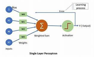
Adaline (Adaptive Linear Neuron) was developed by Professor Bernard Widrow and his student Ted Hoff in 1960 (Adaptive Switching Circuits) at Stanford. It is very similar to a perceptron model. There are some minor differences which include a change in activation function (linear activation), this is followed by a threshold function and thus, the learning is not based on errors from final outputs but is based on the output from activation functions. Following is a diagram of an Adaline neuron:
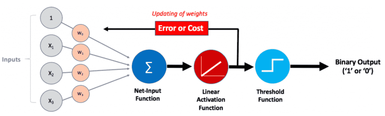
Let's have a look at different steps in the working of an Adaline network:
- Input - It takes input X where X can have any number of dimensions d i.e. x1, x2, x3,...., xd
- Weight matrix - There's a weight w(i) assigned corresponding to each dimension d.
- Weighted sum - The dot product or the weighted sum ( z= Σ d i=1 xiWi = WTX ) is calculated in the next step. We have assumed that W and X are both column/row vectors.
- Activation - This weighted sum is then passed on to the activation function which is just a linear activation that is equivalent to multiplying the aggregated values with 1.
- Weight Update - This step is something that separates Adaline from perceptron neurons. In this step we pass the difference between continuous aggregated value and class label to the model to learn. This is a self-learning step defined by the following equations:
- Thresholding function - This function takes the value from the linear activation function and uses a threshold to predict the final output.
wi := wi + Δwi
where Δwi = η*(targeti - outputi)* x i i
One thing to keep in mind here is that the output here is a continuous value. This means that even if our prediction is correct our model will still try to learn. For example, say our output is 0.8 (for class 1 input) with a threshold of 0.6 but the difference between label value 1 and output 0.8 is 0.2 which indicates that our model will try to bridge the gap between 0.8 and 1.
g(z)= { 1 if z > Θ - 1 otherwise
This sums up the working of an Adaline neuron. In a nutshell, the major difference between Adaline and perceptron is that perceptron uses class labels to learn model coefficients whereas Adaline uses continuous predicted values to learn model coefficients. The method used by Adaline is more powerful as it tells your model how much wrong or right its predictions are.
One of the major issues concerned with both Adaline and perceptron models is that they cannot solve a nonlinear problem (failure on solving an XOR gate problem). Later, the researchers found that such problems can be solved by stacking multiple neurons, which led to the birth of Madaline.
Madaline
Madaline (Many Adaline) is a three-layer (input, hidden, output), fully connected, a feed-forward artificial neural network that uses Adaline neurons in its hidden and output layers. It has multiple Adaline units in parallel in the hidden layer and one Madaline neuron in the output layer. Have a look at the architecture of the Madaline network:
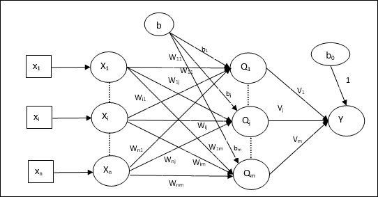
Let's talk about architecture. It consists of 'n' neurons in the input layer, 'm' neurons in the Adaline layer, and 1 neuron in the Madaline layer. Following is a stepwise propagation through this network:
- Input - Input consists of an 'n' dimension vector having input values.
- Net input at a neuron of Adaline layer (fo j Adaline neurons) -
- Output (Qj) from each neuron of the Adaline layer is governed by the function given below -
- The final output is governed by the following equation of weighted sum of input from previous layer and weights from the previous layer to the output neuron:
- Weight update - This stage has three different cases mentioned below:
- Case - 1 (y is not equal to target value, target value = 1)
- Case - 2 (y is not equal to target value, target value = -1)
- Case - 3 (when actual output is equal to target output)
Qinj = b
bj is the bias term, wij is the weight for input neuron i to Adaline hidden neuron j.
f(x) = {1 if x≥0 - 1 if x<0
Qj = f(Qinj)
yinj = b0+ Σ m j=1 Qjvj
y = f(yinj)
wij(new) = w ij(old) + α * (1 - Qinj)xi
bj(new) = bj(old) + α * ( 1 - Qinj)
wik(new) = w ik(old) + α * (1 - Qink)xi
bk(new) = bk(old) + α * ( 1 - Qink)
In this case, there is no change in weights.
Conclusion
This brings us to an end of how the development of artificial neurons took place over the past few decades. This progressive development eventually led to the idea of the modern Neural Network architecture that we see and use nowadays. We went through perceptron, Adaline, and Madaline models where we also discussed the difference between these models. More about the further development of neural nets in the upcoming articles. Happy learning!
References
- https://isl.stanford.edu/~widrow/papers/c1988madalinerule.pdf
- https://sebastianraschka.com/faq/docs/diff-perceptron-adaline-neuralnet.html
- https://cs.stanford.edu/people/eroberts/courses/soco/projects/neural-networks/Neuron/index.html