

Support Vector Machines

Course Lessons
| S.No | Lesson Title |
|---|---|
| 1 | Introduction |
| 2 | Residual Block |
| 2.1 | SVM vs Naïve Bayes |
| 2.2 | SVM vs Logistic Regression |
| 2.3 | SVM vs KNN |
| 3 |
SVM |
| 3.1 | Hyperplane |
| 3.2 | Linearly vs Non-Linearly separable data |
| 3.3 | Support Vectors |
| 3.4 | Maximum Margin Hyperplane |
| 3.5 | C value |
| 3.6 | Kernel Trick in SVM |
| 4 |
Steps involved in making a SVM model |
| 4.1 | Step 1 |
| 4.2 | Step 2 |
| 4.3 | Step 3 |
| 4.4 | Step 4 |
| 4.5 | Step 5 |
| 4.6 | Parameters inside SVM of Sklearn |
| 5 |
Project using SVM |
| 5.1 | Importing and Preproecessing Data |
| 5.2 | Creating Model |
| 5.3 | Hyperparameter Tuning |
| 6 | Conclusion |
Introduction
Support Vector Machine or SVM is a popular supervised machine learning algorithm introduced by Vladimir Vapnik and his colleagues in the late '90s. SVMs are considered to be one of the most robust prediction techniques, which is based on statistical analysis. SVMs can be used for both classification and classification tasks. In the SVM algorithm, we plot each training example (having n features) as a point in an n-1 dimensional hyperplane wherein each feature acts as a value for a particular coordinate. SVM works well for both linearly and nonlinearly separable data. The optimum hyperplane is found using the help of support vectors.
There are many applications of SVM. One of them is the Facial Expression classifier. Using SVM we can make a classifier that can detect whether a person is happy or sad by training on such images. Here, all the images will be converted to features and our SVM model would train on those images to classify happy and sad images.
Another application of SVM is Handwriting classification. SVM model would be able to differentiate between the handwriting of two people. In such a problem our dataset would contain images of the handwriting of two people. We will train our SVM model on these images and it would be able to draw a hyperplane between the two classes.
Comparison of SVM with other machine learning algorithms
SVM VS Naïve Bayes
The difference between the SVM and the Naïve Bayes classifier is from a features point of view. Naïve Bayes treats every feature as independent, whereas SVM sees the interaction between the features to some degree with the help of non-linear kernels (Gaussian, RBF, Poly, etc.). Since SVMs kernels can handle non-linearities in the data, they perform better than Naïve Bayes.
SVM VS Logistic Regression
SVM is a better choice than logistic regression because SVM tries to find the best margin that separates the two classes which reduces the risk of error, while logistic regression does not do that, instead, it can have different decision boundaries with different weights that are near the optimal point. Also, the risk of overfitting is less in SVM as compared to logistic regression.
SVM vs KNN
SVM takes care of outliers better than KNN. If there are a large number of features and less training data then SVM is a better classifier.
SVM
Hyperplane
A hyperplane is a plane of n-1 dimensions in an n-dimensional feature space that is used to separate 2 classes. If the number of features in our dataset is 2 then our hyperplane will only be a line, but if the number of features becomes 3 then we would need a 2-dimensional plane to separate the classes. So in this case, our hyperplane will be a 2D plane.
Let us look at the below figure to get a better understanding of the hyperplane.
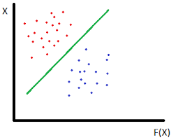
This is a dataset that has 2 classes of data. It has 2 features hence it is plotted on a 2-dimensional plane. To classify between them we need a hyperplane (which in this case is a line) that passes between the two classes.
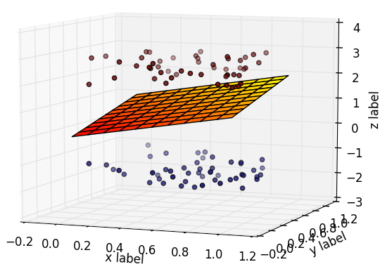
This is a dataset that has 2 classes of data. It has 3 features hence it is plotted on a 3-dimensional plane. To classify between them we need a hyperplane (which in this case is a plane) that passes between the two classes.
Hyperplanes with 3 or more dimensions are difficult to portray or visualize.
Linearly vs Non-Linearly separable data
A dataset is said to be linearly separable if we can draw a straight hyperplane to classify the classes and a dataset where the classes can not separate by a straight line is referred to as non-linear data.
Now we will try to visualize linearly and nonlinearly separable datasets. To visualize linearly separable data we will use the make_blobs method inside the sklearn library and to visualize the non-linearly separable data, we will use the make circles method inside sklearn. SVM can find a decision boundary for non-linearly separable very accurately, which is because of the presence of kernels in SVM.
# Let us make a linearly separable data. The make_blobs library helps to make
#clusters of data points

from sklearn.datasets import make_blobs
import matplotlib.pyplot as plt

# Here we are making 2 clusters which can be seen by the 'centers' parameter.
# Every data point will have 2 features.
#500 such points will be generated with equal number of data points belonging to
#each class.

x,y  = make_blobs(n_samples=500,n_features=2,centers=2,random_state=3)

#Now that the clusters are made we can plot them using scatter funtion in matplotlib.
# The first parameter is the first feature in x matrix and second argument is the
#second feature in the x matrix.
# color of each cluster is going to be decided using the total number of classes, i.e 2

plt.scatter(x[:,0],x[:,1],c=y,cmap=plt.cm.Accent)
plt.show()
Output:
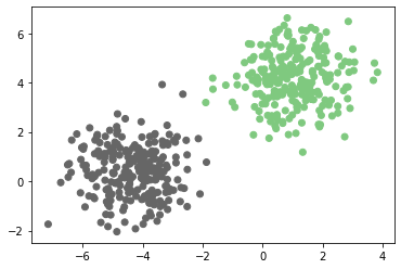
This is linearly separable data as it can be separated using a linear hyperplane (in this case a line).
# Let us now make a non- linearly separable data. The make_circles library helps to make concentric of data points

from sklearn.datasets import make_circles
import matplotlib.pyplot as plt

# Here we are making 2 concentric circles
#500 such points will be generated with equal number of data points belonging to each class.

x,y  = make_circles(n_samples=500, shuffle=True, noise=0.2, random_state=1, factor=0.2)


#Now that the circles are made we can plot them using scatter funtion in matplotlib.
# The first parameter is the first feature in x matrix and second argument is the second feature in the x matrix.
# color of each concentric circle is going to be decided using the total number of classes, i.e 2

plt.scatter(x[:,0],x[:,1],c=y,cmap=plt.cm.Accent)
plt.show()
Output:
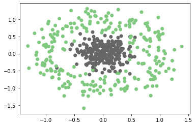
This is non-linearly separable data and we can not draw a linear hyperplane to classify these points. In this case, our hyperplane needs to be a circle.
Support Vectors
Support vectors are the points that are closest to the hyperplane. They play a major role in deciding the position and orientation of the hyperplane. Support vectors help to maximize the margin of the classifier.
Maximum Margin Hyperplane
The goal in SVM is to find the maximum margin hyperplane. It means we have to find a hyperplane, which is farthest from the closest points of both the classes.
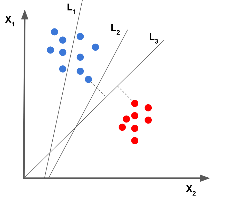
In this figure, line 3 is the maximum margin hyperplane as it is farthest from the support vectors of both the classes.
We want our predictions to be confident and correct.Meaning of confidence can be understood from below example.
Let a,b,c, be 3 points from a hyperplane.
D1= Distance of point 'a' from hyperplane
D2= Distance of point 'b' from hyperplane
D3= Distance of point 'c' from hyperplane
And D1 = 1 unit, D2 = 2 units and D3 = 3 units.
So, we are more confident about D3 as it is the farthest from the hyperplane.
C Value
To get a better classification SVM looks for a maximum margin hyperplane. That is where 'C' comes into the picture. 'C' is the penalty parameter of the error term. A small value of C gives a large margin, which means that there will be some misclassification but it will result in higher accuracy on our test data. A large value of C gives a small margin, which means that there will be little to no misclassification, but it will result in lower accuracy on our test data. In general, we should keep our C value low. The optimum value of C for a particular project is decided using hyperparameter tuning.
Kernel Trick in SVM
One of the main advantages that make SVM stand out from other classifiers is that the different kernels it offers. Kernels allow us to project our n-dimensional data on a higher feature space while still operating on the n-dimensional feature space. It means that with the help of kernels we can project 2d data to 3 or more dimensions which makes it easier for the classifier to find an optimum hyperplane, particularly for non-linearly separable data.
Below are the list of some of the kernels that SVM has:
- Linear Kernel: A linear kernel is used when we have linearly separable data. It is one of the most commonly used kernels and is mostly used when there are a large number of features in a particular dataset.
- Polynomial Kernel: It transforms our dataset into a higher degree polynomial.
- RBF Kernel: Radial basis function (RBF) kernel is used mainly when data is non-linearly separable.
Now let us look at the svm classifier in sklearn.
# Here we are making a dataset belonging to 2 classes which are 0 and 1.
# The dataset has 1000 training points which can be seen from n_samples parameter.
#Every point has 2 features which can be seen from the n_featues parameter


from sklearn.datasets import make_classification
import matplotlib.pyplot as plt

X,Y=make_classification(n_samples=1000,n_classes=2,n_features=2,n_informative=2,n_redundant=0,random_state=1)
Steps involved in making a SVM Model
Step 1:
We have to start by importing the dataset, and this can be in the form of a CSV file, excel sheet, or even text file. In this example, we are creating a dummy dataset using the sklearn make_classification method.
Step 2:
We have to perform Exploratory Data Analysis or EDA. In this we visualize the data, clean the data and check for imbalances in the data among other things. Since in this example we have just generated dummy data so we don't have to clean the data or check for any imbalances. We can just visualize it.
# Here we are visualising our dataset using scatter method in matplotlib.pyplot
# The first parameter is the x coordinate of our graph and the second parameter is the y coordinate.
# color of each class is going to be decided using the number of classes in Y matrix, i.e 2

plt.scatter(X[:,0],X[:,1],c=Y,cmap=plt.cm.Accent)
plt.plot()
Output:

Step 3:
Now we make a SVM classifier.
# Here we are importing the svm classifier from sklearn

from sklearn import svm

# SVC stands for Support Vector Classifier.
# Here we aren't specifying any parameters inside SVC object. By default SVC has C values as 1.0 and kernel is 'rbf'

svc= svm.SVC()

# Now we are training our classifier on our dummy dataset.

svc.fit(X,Y)
Output:
 SVC(C=1.0, break_ties=False, cache_size=200, class_weight=None, coef0=0.0,
        decision_function_shape='ovr', degree=3, gamma='scale', kernel='rbf',
        max_iter=-1, probability=False, random_state=None, shrinking=True,
        tol=0.001, verbose=False)
Our model is now trained.
Step 4:
Now we will test our classifier.
# we are testing our classifier for a dummy point (0,0).
z=svc.predict([[0,0]])
print(z)
Output:
[0]
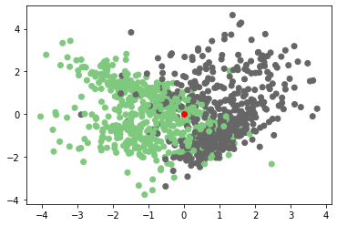
The classifier is predicting that it belongs to 0th class and we can also visualise this prediction.
# Here we are visualising our original dataset  along with the test point (0,0).
#The test point will have red color

plt.scatter(X[:,0],X[:,1],c=Y,cmap=plt.cm.Accent)
plt.scatter(0,0,c='red')
plt.plot()
Output:
Step 5:
After we have made a base model we can start improving our accuracy using hyperparameter tuning.
Parameters inside SVM of SKLearn
NOw we will learn about all the parameters inside SVM classifier of sklearn
- C: It is a regularization parameter. It must be strictly positive. It's default value is 1.0
- Kernel: This parameter specifies the kernel that should be used in the classifier. Its default value is 'rbf'.
- degree: It provides the degree of polynomial kernel. It's default value is 3. It is ignored by all other kernels
- gamma: It provides the kernel coefficient for 'rbf' 'poly' and 'sigmoid' kernels. If gamma='scale' which is the default value then it used 1/(n_features*X.var()) as gamma. If it's auto then it uses 1/n_features.
- coef0: It is the independent term in the kernel function. It is only significant for 'poly' and 'sigmoid' kernels. Its default value is 0.0
- shrinking: It is a boolean variable and defines whether to use the shrinking heuristic. Its default value is True.
- probability: It is a boolean value and it defines whether to enable the probability estimates. Its default value is False. This must be enabled prior to calling fit function.
- tol: It is the tolerance for stopping criterion. It's default value is 1e-3.
- cache_size: It specifies the size of the kernel cache (in MB). It's default value is 200.
- class_weightdict or 'balanced', default = None : It sets the parameter C of class i to class_weight[i]*C for SVC. If not given, all classes are supposed to have weight one. Its default value is None.
- verbose: It is a boolean variable which enables the verbose output. Its default value is False.
- max_iter: It is the hard limit on iterations. Its default value is -1.
- decision_function_shape: This parameter states whether to return a one-vs-rest ('ovr') decision function of shape (n_samples, n_classes) as all other classifiers, or one-vs-one ('ovo') decision function which has shape (n_samples, n_classes * (n_classes - 1) / 2). Its default value is 'ovr' and is ignored for binary classification.
- random_state: It controls the pseudo random number generation for shuffling the data for probability estimates. Its default value is None.
Project using SVM
We will now see a Classification problem is solved using an SVM model. In this example, we will be predicting whether a given person has Parkinson's disease or not. In this, we have a dataset of 195 patients having many attributes. The final attribute is status which is our target variable. The status has 2 values 0(patient does not have Parkinson's disease) or 1(patient has Parkinson's disease). This is a binary classification problem.
Importing and Preproecessing Data
We will start by importing all the libraries we need for this project.
# Here we are importing all the necessary libraries for our project

import numpy as np
import pandas as pd
import matplotlib.pyplot as plt
import seaborn as sns

# The train_test_split from sklearn library helps us to divide our data into training and test set

from sklearn.model_selection import train_test_split

#Here we are importing the SVM model from sklearn

from sklearn import svm

# GridSearchCV will help us in hyperparameter tuning

from sklearn.model_selection import GridSearchCV
Using the above code we have imported all the libraries that we needed. Now we will import our data which is available in .csv format and store it in a Pandas dataframe.
# Here we are reading our data which is in .csv format
#and we are making a Pandas dataframe out of it
#and storing it in a variable named df.

df=pd.read_csv('parkinsons2.csv')
# This will show the first 5 rows of our dataset, unless specified otherwise
df.head()Output:
| MDVP:Fo(Hz) | MDVP:Fhi(Hz) | MDVP:Flo(Hz) | MDVP:Jitter(%) | MDVP:Jitter(Abs) | MDVP:RAP | MDVP:PPQ |
|---|---|---|---|---|---|---|
| 119.992 | 157.302 | 74.997 | 0.00784 | 0.00007 | 0.0037 | 0.00554 |
| 122.4 | 148.65 | 113.819 | 0.00968 | 0.00008 | 0.00465 | 0.00696 |
| 116.682 | 131.111 | 111.555 | 0.0105 | 0.00009 | 0.00544 | 0.00781 |
| 116.676 | 137.871 | 111.366 | 0.00997 | 0.00009 | 0.00502 | 0.00698 |
| 116.014 | 141.781 | 110.655 | 0.01284 | 0.00011 | 0.00655 | 0.00908 |
As we can see our dataset has 23 attributes. The last attribute is our target variable which is status. We will move our target variable out of the dataset and into a separate variable
Let us now display the type of columns present in our dataset.
# This will display information about all the columns in our dataset.

df.info()
Output:
<class 'pandas.core.frame.DataFrame'>
RangeIndex: 195 entries, 0 to 194
Data columns (total 23 columns):
MDVP:Fo(Hz)         195 non-null float64
MDVP:Fhi(Hz)        195 non-null float64
MDVP:Flo(Hz)        195 non-null float64
MDVP:Jitter(%)      195 non-null float64
MDVP:Jitter(Abs)    195 non-null float64
MDVP:RAP            195 non-null float64
MDVP:PPQ            195 non-null float64
Jitter:DDP          195 non-null float64
MDVP:Shimmer        195 non-null float64
MDVP:Shimmer(dB)    195 non-null float64
Shimmer:APQ3        195 non-null float64
Shimmer:APQ5        195 non-null float64
MDVP:APQ            195 non-null float64
Shimmer:DDA         195 non-null float64
NHR                 195 non-null float64
HNR                 195 non-null float64
RPDE                195 non-null float64
DFA                 195 non-null float64
spread1             195 non-null float64
spread2             195 non-null float64
D2                  195 non-null float64
PPE                 195 non-null float64
status              195 non-null int64
dtypes: float64(22), int64(1)
memory usage: 35.2 KB
From the output we have the following observations:
- There are 195 data points in our dataset.
- All the attributes are of type float64
- The target variable, i.e. 'status' is of type int64
- There are no null values in our dataset which means that the data is already cleaned. So we can directly start building our model.
We will now move our target variable in a separate variable.
# Here we are moving our status variable which is our target variable into a separate variable

y=df.status

#Here we are dropping out the status variable from the DataFrame.

df.drop(['status'],axis=1,inplace=True)
We have now moved our target variable i.e, status, in a separate variable 'y' and we have dropped the status variable from our dataframe.
Now we will find the correlation matrix and will plot the heatmap to see the relationship between variables.
#Here we are creating a correlation matrix and a heatmap

corr = df.corr()
plt.subplots(figsize=(30,10))
sns.heatmap( corr, square=True, annot=True,fmt=".1f")
Output:
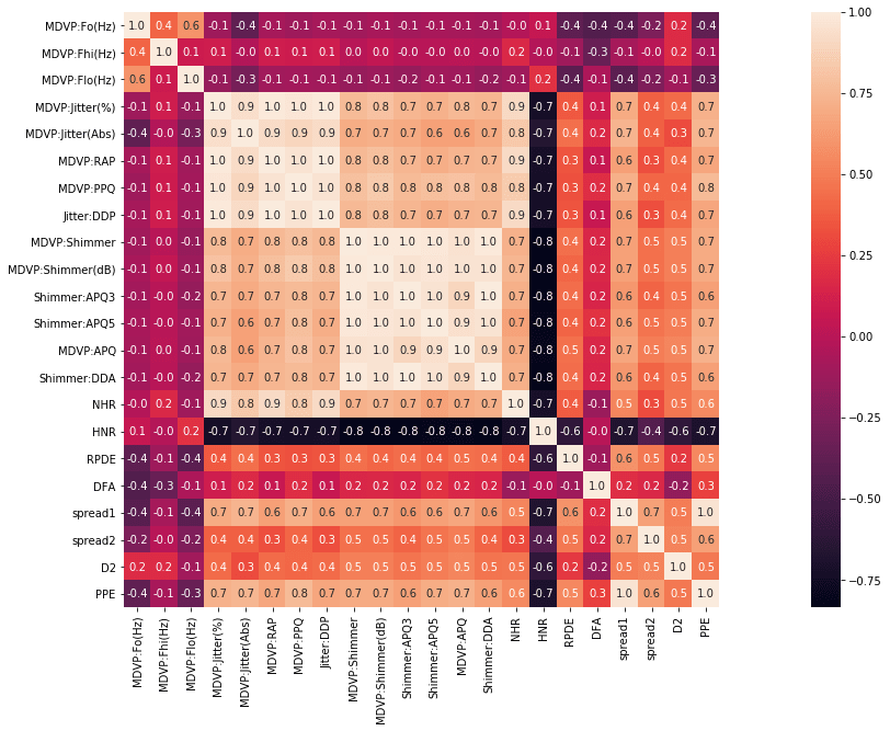
The blocks that are shaded lighter mean that they have higher degree of relation.
We will now split our data into training and test sets.
# Here we are splitting our dataset into training and test sets. 33% of our data will be in the test set and the rest of the data will be used for training

X_train, X_test, y_train, y_test = train_test_split(df,
                                                    y,
                                                    test_size=0.33,
                                                    random_state=42)
Creating Model
The next step is to create a SVM model and train our data.
#Here we are making a SVM classifier. We haven't defined any parameter in our classifier, so the default values will be taken for training  which is C=1.0 and kernel='rbf'.
svc = svm.SVC()
svc.fit(X_train,y_train)
Output:
SVC(C=1.0, break_ties=False, cache_size=200, class_weight=None, coef0=0.0,
        decision_function_shape='ovr', degree=3, gamma='scale', kernel='rbf',
        max_iter=-1, probability=False, random_state=None, shrinking=True,
        tol=0.001, verbose=False)
As we can see our model is now trained with C=1.0 and kernel='rbf'
Now we have to test our model.
# Here we are calculating the score of our model with the help of our test data.

svc.score(X_test,y_test)
Output:
0.7846153846153846
The model achieved a score of 78.46% on the test data.
Hyperparameter Tuning
This is our base model. We will now use hyperparameter tuning to get better accuracy. The hyperparameters that we are going to tune are kernel and C values. We are going to use GridSearchCV to tune our parameters. For the kernel, we are taking 'linear', 'rbf', 'poly', and 'sigmoid' kernels. For C value we are taking 0.1, 0.2, 0.5, 1.0, 2.0, 5.0.
# Here we are defining a list of parameters that we are going to be tuning using GridSearchCV
# for kernel we are taking 'linear','rbf','poly' and 'sigmoid'
#for C value we are taking 0.1, 0.2, 0.5, 1.0, 2.0, 5.0
#GridSearchCV will explore all the possible combinations of these parameter and will give us the model which performed the best

params = [
    {
        'kernel':['linear','rbf','poly','sigmoid'],
        'C':[0.1,0.2,0.5,1.0,2.0,5.0]
    }
]
Output:
8
From the output we can see that we have 8 CPUs which means that we can run 8 jobs in parallel
Now we will find the best hyperparameters using GridSearchCV.
#Here we are finding the best hyperparameters.
#Our estimator is the SVM object.
# The parameters are the grid defined above.
# We are performing 5 fold cross validation.

gs = GridSearchCV(estimator=svm.SVC(),param_grid=params,scoring="accuracy",cv=5,n_jobs = cpus)

#Here we are training our GridSearchCV model.

gs.fit(X_train,y_train)

# Here we are outputting the parameter of the best estimator

gs.best_estimator_
Output:
SVC(C=0.5, break_ties=False, cache_size=200, class_weight=None, coef0=0.0,
        decision_function_shape='ovr', degree=3, gamma='scale', kernel='linear',
        max_iter=-1, probability=False, random_state=None, shrinking=True,
        tol=0.001, verbose=False)
Using GridSearchCV we have found the best parameters for our SVM model.As we can see the best accuracy is achieved when we have C=0.5 and kernel='linear'.So, now let us make another SVM object with the above parameters.
#Now we are making a new SVM classifier with C=0.5 and kernel='linear' as these were the values which we calculated by GridSearchCV to have the best result for our classifier.

svc=svm.SVC(C=0.5,kernel='linear')

#Here we are training our model

svc.fit(X_train,y_train)
Output:
SVC(C=0.5, break_ties=False, cache_size=200, class_weight=None, coef0=0.0,
        decision_function_shape='ovr', degree=3, gamma='scale', kernel='linear',
        max_iter=-1, probability=False, random_state=None, shrinking=True,
        tol=0.001, verbose=False)
As we can see that our model is now trained after hyperparameter tuning. As calculated by GridSearchCV we have used C=0.5 and kernel='linear'.
Now we will test our model and see if our accuracy has improved or not.
svc.score(X_test, y_test)Output:
0.8461538461538461
As we can see that using the Hyperparameters as found by GridSearchCV we were able to increase our accuracy from 78.46% to 84.61%.
Conclusion
In this article, we have studied the working of an SVM classifier. We saw its comparison with some other popular machine learning algorithms. We learned how to create and plot linearly and non-linearly separable data using sklearn. We learned about different kernels in SVM. Finally, we made an SVM model which can detect whether a person has Parkinson's disease or not, in which we learned how to use GridSearchCV to find the best hyperparameter for our SVM classifier.