

Principal Component Analysis
Course Lessons
"We prefer to listen to a concise explanation of a story than a lengthy and complicated one. Even the predictive models expect the same, the curated low dimensional data than having sparse high dimensional data."
1. Introduction
Dimension refers to the number of input features/attributes or variables. Dimensionality reduction involves reducing the number of features of a dataset to form a subset that represents the original high-dimensional data. High dimensional data often imposes numerous challenges on predictive models, generally referred to as the "Curse of dimensionality" as quoted by the mathematician Richard Bellman. To be more specific, as the dimension of the data increases, the complexity level of analyzing, organizing, and visualizing the data increases. In the next section, we will discuss the shortcomings of high-dimensional data followed by the method to efficiently reduce the dimension of the data.
1.1 Challenges Faced By High-Dimensioned Feature Sets
Some of the challenges faced by high-dimensioned feature sets are as follows:
- The large datasets cause high computation time and memory overhead during the training process.
- Making the model account for so many features or variables to make a decision may induce poor real-time performance.
- The complexity of the model needs to be increased when dealing with the high-dimensional data, leading to overfitting and poor generalizability.
- The features may have correlations and hence the model will have bias towards correlated features and results may be unreliable.
"When dealing with high dimensional data, it is often useful to reduce the dimensionality by projecting the data to a lower dimensional subspace which captures the "essence" of the data. This is called dimensionality reduction."
- Machine Learning: A Probabilistic Perspective (Adaptive Computation and Machine Learning series)
Now that we know the challenges associated with the high-dimensional data; think of a method that summarizes and generates the subset of the dataset representing the original high-dimensional data that can be easily analyzed. This is where Principal Component Analysis (PCA) comes into play. In the next section, we will walk through the working of PCA.
"Dimensionality reduction yields a more compact, more easily interpretable representation of the target concept, focusing the user's attention on the most relevant variables"
2. Principal Component Analysis (PCA)
Principal Component Analysis (PCA) is a method derived from linear algebra intended for significantly reducing the number of dimensions in a dataset while retaining most of the important information. PCA is widely used in the domain of machine learning, pattern recognition, and signal processing for preparing the dataset to create a projection of a dataset before fitting a model. In PCA, we create a set of Principal Components or new features from the Input dataset by solving an Eigenvector/Eigenvalue problem. The Principal Components capture the most important information from the dataset to reduce the loss of data while reducing dimensions. In PCA, we are trying to project our points on a suitable hyperplane to reduce our dimensions. For example, if we want to reduce our dimensions from 3 to 2, then we would need to project our data points present in the 3D coordinate system to a 2D hyperplane. We would take the hyperplane which would give the most variance in our data, to retain most of the information.
2.1 Steps in PCA
Let us now get a brief idea on the steps involved in PCA after that we will take a closer look at all the steps.
- We are going to compute a matrix that will summarize how our variables relate to each other.
- We will then break down this matrix into direction and magnitude, which will help us to understand the importance of each direction.
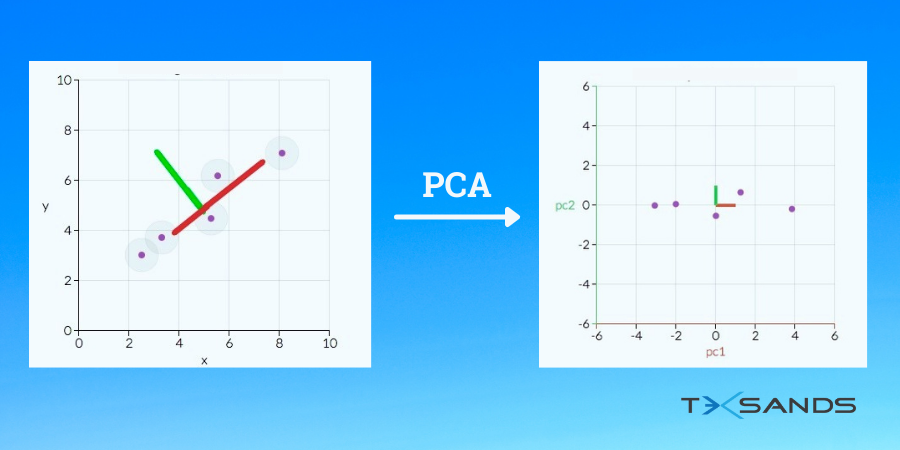
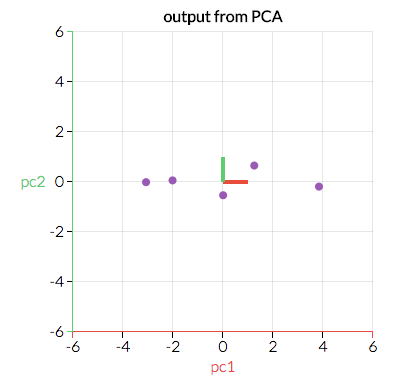
- Now, we have to see what would be the best fit line. We need to reduce the features of our data in such a way that we get the maximum amount of variance in our new reduced dataset. This can be seen by plotting our data on both the lines and see how much variance we get in our new dataset when it is projected on both the lines.
- If we project our points on the red line we will see that the distance between the points in the red line is more than in the green line. So, the red line is the best line to protect our data on.
- Now we will transform our data in such a way that it is aligned with the red line.
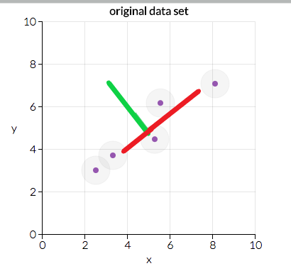
Here we can see two directions which are the red and green lines. We will transform our data in such a way that it is projected on the best line.
Now let us take an in-depth look at all the steps involved in PCA. Steps involved in performing PCA are as follows:
- Standardization of Data
- Obtaining the covariance matrix
- Calculating the Eigenvectors and Eigenvalues
- Computing the Principal Components
3. PCA On MNIST Data
To understand the working of PCA, we will perform every step on the MNIST dataset by using the keras framework. MNIST dataset has 784 features, but we will reduce the number of features to 2 using PCA.
3.1 Standardization
Standardization is a feature scaling technique where the values are centered around the mean with a standard deviation of 1. This means that the mean of the attribute will become 0, and the new distribution will have a standard deviation of 1.
Let us perform standardization on MNIST dataset.
#Here we are importing the MNIST dataset from keras and making loading train and test data from it

from keras.datasets import mnist

(X_train,Y_train),(X_test,Y_test)=mnist.load_data()

#We are only performing PCA on the train data right now

# Now let us reshape our train data

X=X_train.reshape(-1,28*28)
Y=Y_train

#Now let us import StandardScaler from Sklearn and Standardize our dataset

from sklearn.preprocessing import StandardScaler

sc=StandardScaler()

#We are Standardizing our train data and storing it in a variable X_

X_=sc.fit_transform(X)
The training data is now standardized and now it has 10000 rows (training samples) and 784 columns (features).
3.2 Obtaining The Covariance Matrix
Now our task is to obtain the covariance matrix for our dataset.
The covariance matrix will help us to determine how our features relate to one another. The covariance matrix is obtained by multiplying the standardized matrix X_ and its transpose X_T. Since our dataset has 784 features, our covariance matrix will be of the shape (784,784).
#Let us import numpy and compute the covariance matrix

import numpy as np

#Now let use calculate the covariance matrix.

covar=np.dot(X_.T,X_)

covar.shape
Output: (784, 784)
As we can see our covariance matrix has the shape of (784,784).
3.3 Calculating Eigenvectors and Eigenvalues
Now we have to calculate eigenvectors and their corresponding eigenvalues of our covariance matrix. Calculating eigenvectors and eigenvalues are important for the following reason:
We need to find the best fit line, on which we can project our dataset and can have maximum variance. The eigenvector indicates the direction of that line, and the eigenvalue is a value that tells us how the data is spread out on the line.
We will decompose our covariance matrix X_TX_ into PDP-1 where P is the matrix of eigenvectors and D is the diagonal matrix with the eigenvalues situated at the diagonals and 0 at every other position.
The above task of calculating eigenvectors can be achieved through Singular Value Decomposition (SVD) from numpy. This function will return 3 values, The first of which will be our eigenvectors.
#Let us import svd from numpy

from numpy.linalg import svd

#Here we are feeding our SVD function our covariance matrix. SVD will return 3 values u,s,v. Our eigenvectors will be in u.

u,s,v=svd(covar)

u.shape
Output: (784, 784)
Matrix U is a n x n matrix, where n is the number of total dimensions/principal components. We choose the first k columns of the matrix, which represent k dimensions we need.
Now, since we want to reduce our 784 features to 2 features, we will take the first 2 features of the 'u' matrix.
# Here we are extracting the first 2 columns of our u matrix and storing it in a variable call ured

ured=u[:,:2]

ured.shape
Output: (784, 2)
As we can see we have extracted the first 2 features.
3.4 Computing the Principal Components
In this step, we will convert our train data which is of shape (10000,784) to (10000,2). So we will reduce our features from 784 to 2. This will be achieved by multiplying our train data with the Eigenvectors computed above.
z=np.dot(X_,ured)

z.shape
Output: (10000, 2)
As we can see the dimensions of our dataset have been reduced from (10000,784) to (10000,2). Now let us see our reduced dataset.
# We will make a dataframe of our reduced data in order to see it better.

import pandas as pd

#Here we are horizontally stacking our dataset along with our target values

new_data=np.hstack((z,Y.reshape(-1,1)))

#Here we are labelling each column. Feature 1 is PC1 and Feature 2 is PC2.

dataframe=pd.DataFrame(new_data,columns=['PC1','PC2','label'])

dataframe.head()
| PC1 | PC2 | Label | ||
|---|---|---|---|---|
| 0 | 5.45831 | -6.414 | 7 | |
| 1 | -2.8044 | 8.02885 | 2 | |
| 2 | 7.41124 | 3.86404 | 1 | |
| 3 | -8.7512 | -0.046 | 0 | |
| 4 | 0.06576 | -6.2963 | 4 |
As we can see our dataset has now been converted to 2 features.
4. Practical Example
To demonstrate the working of PCA, we will take the House Prices Dataset. We intend to perform a House Price Prediction study. The model will train on various features of previous transactions and associated prices. The Linear Regression algorithm can be used to create the model to predict future property prices.
However, this input comes with 81 fields. That's a very large number of predictor features and will make the model complex. We intend to perform Principal Component Analysis on this dataset to create a small set of derived features that would still include all the information that is required to create an effective model. This set of features can then be taken into the Linear Regression algorithm to build the prediction model.
4.1 Importing Data
The first step is to import all the libraries we require.
  # Import Libraries

import numpy as np
import pandas as pd
import matplotlib.pyplot as plt
import seaborn as sns
from sklearn.decomposition import PCA
import sklearn
from sklearn.preprocessing import MinMaxScaler
import warnings
warnings.filterwarnings('ignore')
Let us now import the dataset into a DataFrame.
# Here we are importing our dataset into a variable called houseprice

houseprice = pd.read_csv("HousePrice.csv", encoding ="utf-8")
houseprice
Output:
| Unnamed: 0 | Id | MSSubClass | MSZoning | LotFrontage | LotArea | Street | Alley | LotShape | LandContour | Utilities | LotConfig |
|---|---|---|---|---|---|---|---|---|---|---|---|
| 0 | 1 | 60 | RL | 65 | 8450 | Pave | Reg | Lvl | AllPub | Inside | |
| 1 | 2 | 20 | RL | 80 | 9600 | Pave | Reg | Lvl | AllPub | FR2 | |
| 2 | 3 | 60 | RL | 68 | 11250 | Pave | IR1 | Lvl | AllPub | Inside | |
| 3 | 4 | 70 | RL | 60 | 9550 | Pave | IR1 | Lvl | AllPub | Corner | |
| 4 | 5 | 60 | RL | 84 | 14260 | Pave | IR1 | Lvl | AllPub | FR2 |
5 rows × 62 columns
As we can see that our dataset has 62 columns
4.2 Exploratory Data Analysis
We need to understand the feature types in the DataFrame. The kind of Preprocessing we have to undertake will depend on that.
houseprice.info()
< class 'pandas.core.frame.DataFrame'>
RangeIndex: 1460 entries, 0 to 1459
Data columns (total 62 columns):
Unnamed: 0       1460 non-null object
Unnamed: 0.1     1460 non-null int64
Id               1460 non-null int64
MSSubClass       1460 non-null int64
MSZoning         1460 non-null object
LotFrontage      1201 non-null float64
LotArea          1460 non-null int64
Street           1460 non-null object
Alley            91 non-null object
LotShape         1460 non-null object
LandContour      1460 non-null object
Utilities        1460 non-null object
LotConfig        1460 non-null object
LandSlope        1460 non-null object
Neighborhood     1460 non-null object
OverallQual      1460 non-null int64
OverallCond      1460 non-null int64
YearBuilt        1460 non-null int64
YearRemodAdd     1460 non-null int64
RoofStyle        1460 non-null object
MasVnrArea       1452 non-null float64
ExterQual        1460 non-null object
ExterCond        1460 non-null object
BsmtFinSF1       1460 non-null int64
BsmtFinSF2       1460 non-null int64
There are a lot of Textual fields(Objects) in our dataset. They cant be read into the model and hence must be converted into meaningful numeric fields
Let us now check for Missing values:
# Check variables for Nulls

houseprice.isnull().sum().sort_values(ascending=False).head(15)
Output:
PoolQC          1453
Alley           1369
FireplaceQu      690
LotFrontage      259
GarageFinish      81
GarageQual        81
GarageCond        81
GarageYrBlt       81
MasVnrArea         8
ExterQual          0
Neighborhood       0
RoofStyle          0
ExterCond          0
BsmtFinSF1         0
YearRemodAdd       0
dtype: int64
The features PoolQC, Alley, FireplaceQu, LotFrontage have a lot of missing values. This is reducing the importance of these features. Hence we will drop these features.
# Drop fields with High Null values

houseprice = houseprice.drop(['PoolQC', 'Alley', 'FireplaceQu', 'LotFrontage'], axis=1)
Drop 'I' field as it doesn't influence the House Price, it's only a record identifier:
houseprice = houseprice.drop(['Id'], axis=1)
The next step is to convert the textual/categorical features into numeric ones. There are two methods that we use:
- For categorical values that have a degree associated with them, we encode them by an increasing numeric value.
- For categorical values that do not have any degree associated, we perform a 'one-hot encoding' creating corresponding Dummy variables
Converting Features with Degree:
# Map ordinal variables to discreet numeric values

houseprice['MSZoning'] = houseprice['MSZoning'].map({'C (All)': 0, 'FV': 1, 'RH': 2, 'RL': 3, 'RM': 4})

houseprice['LandSlope'] = houseprice['LandSlope'].map({'Gtl': 0, 'Mod': 1, 'Sev': 2})

houseprice['ExterQual'] = houseprice['ExterQual'].map({'Po': 0, 'Fa': 1, 'TA': 2, 'Gd': 3, 'Ex': 4})

houseprice['ExterCond'] = houseprice['ExterCond'].map({'Po': 0, 'Fa': 1, 'TA': 2, 'Gd': 3, 'Ex': 4})

houseprice['HeatingQC'] = houseprice['HeatingQC'].map({'Po': 0, 'Fa': 1, 'TA': 2, 'Gd': 3, 'Ex': 4})

houseprice['CentralAir'] = houseprice['CentralAir'].map({'Y': 0, 'N': 1})

houseprice['KitchenQual'] = houseprice['KitchenQual'].map({'Po': 0, 'Fa': 1, 'TA': 2, 'Gd': 3, 'Ex': 4})

houseprice['GarageFinish'] = houseprice['GarageFinish'].map({'NA': 0, 'Unf': 1, 'RFn': 2, 'Fin': 3})

houseprice['GarageQual'] = houseprice['GarageQual'].map({'Po': 0, 'Fa': 1, 'TA': 2, 'Gd': 3, 'Ex': 4})

houseprice['GarageCond'] = houseprice['GarageCond'].map({'Po': 0, 'Fa': 1, 'TA': 2, 'Gd': 3, 'Ex': 4})
For the categorical features without a degree, we will create one hot encoding.
# Create Dummy Variables for Categorical-Nominal Variables

varsforDummy = ['Street', 'LotShape', 'LandContour', 'Utilities', 'LotConfig', 'Neighborhood', 'RoofStyle', 'Heating', 'PavedDrive']

houseprice = pd.get_dummies(houseprice, columns = varsforDummy, drop_first = True)
Once we have the transformation of the Textual Categorical features sorted, we have another step, Standardization to perform. The Standardization step will convert the numeric values within the features into a standard scale. The original dataset has features that are on a different scale and features with a larger scale will have an undesired higher influence on the derivation of the Principal Components. The features input to the PCA process must be brought at the same scale through Standardization
# Scale the Numeric Variables - use the Min-Max / Normalization method of Scaling

all_cols = houseprice.columns

scaler = MinMaxScaler()

houseprice[all_cols] = scaler.fit_transform(houseprice)
Now that we have the Standardization of data done, we are ready to perform our PCA. Before we go ahead, we have to split the DataFrame into the target and predictor features.
# Create the X_train (predictor variable set) and y_train (target variable set)

y = houseprice.pop('SalePrice')

X = houseprice

X
Output:
| MSSubClass | MSZoning | LotArea | LandSlope | LotFrontage | OverallQual | OverallCond | YearBuilt | YearRemodAdd | LandContour |
|---|---|---|---|---|---|---|---|---|---|
| 0 | 0.235294 | 0.666667 | 0.03342 | 0 | 0.666667 | 0.5 | 0.949275 | 0.883333 | 0.1225 |
| 1 | 0 | 0.666667 | 0.038795 | 0 | 0.555556 | 0.875 | 0.753623 | 0.433333 | 0 |
| 2 | 0.235294 | 0.666667 | 0.046507 | 0 | 0.666667 | 0.5 | 0.934783 | 0.866667 | 0.10125 |
| 3 | 0.294118 | 0.038561 | 0.038561 | 0 | 0.666667 | 0.5 | 0.311594 | 0.333333 | 0 |
| 4 | 0.235294 | 0.666667 | 0.060576 | 0 | 0.777778 | 0.5 | 0.927536 | 0.833333 | 0.21875 |
The above data shows that all our values are now in the range 0-1.
4.3 PCA
As the first step towards performing PCA, we create an object of type PCA and 'fit' the predictor features. We are limiting the PCA to 40 components. The rationale behind 40 components is that we have already iterated a few times with different values of n_components and 40 components roughly explain 90% of the data variance which is decent.
pca = PCA(random_state=100, n_components=40)

pca.fit(X)
Output:
PCA(copy=True, iterated_power='auto', n_components=40, random_state=100,

svd_solver='auto', tol=0.0, whiten=False)
Printing the Principal Components. Principal axes in feature space, representing the directions of maximum variance in the data. The components are sorted by explained_variance_.
pca.components_
Output:
array([[ 1.64838067e-02,  8.02437311e-02, -1.11982823e-02, ...,
6.12264874e-03,  3.41843357e-02, -1.46312291e-01],
[-8.44601563e-02,  2.81142939e-02,  8.34655678e-03, ...,
1.15928788e-04,  1.75158544e-03, -2.16444039e-02],
[-7.23189984e-02,  3.95209530e-02,  2.02969279e-02, ...,
8.14608176e-04,  4.42426183e-03, -2.22358428e-02],
...,
[-1.78650232e-02, -1.02373406e-01, -1.08968597e-02, ...,
1.30213359e-02,  2.40800538e-01,  2.56673770e-02],
[-3.50197536e-02, -3.21968452e-02, -1.78078591e-02, ...,
1.38228502e-02,  3.87850780e-02,  8.35435156e-02],
[ 2.25941593e-02,  3.89966300e-02, -1.94527083e-03, ...,
-2.18023111e-03,  8.96040700e-02,  5.01139594e-02]])
Printing the Explained Variance Ratio: Percentage of variance explained by each of the selected components.
pca.explained_variance_ratio_Print other Attributes to understand the PCA better.
print("n_components_", pca.n_components_)

print("n_features_", pca.n_features_)

print("n_samples_", pca.n_samples_)
Output:
Now we plot a Bar plot with the values of how much variance in the training data is explained by each Principal Component. This is plotted in decreasing order of variance explained percentage.
# Bar Plot to display how much percentage of overall (100%) variance is explained by each Principal Component

plt.bar(range(1,len(pca.explained_variance_ratio_)+1), pca.explained_variance_ratio_)
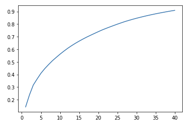
#Here we are taking the cumulative sum of the explained_variance_ratio, in order to understand how much percentage of variance can be explained by every combination of features

var_cumu = np.cumsum(pca.explained_variance_ratio_)
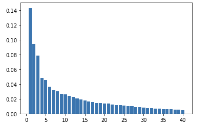
The X-axis is the sequence of Principal Components and the Y-axis is the %age of variance explained by the corresponding Principal Component.
All Principal Components together explain 100% variance.
We also plot the 'Scree Plot' to make a little better visually to show 40 components that we have selected actually explain 90% of the variance.
# Scree plot

plt.plot(range(1,len(var_cumu)+1), var_cumu)
Output:
Once the PCA is completed, we would be interested to obtain the dataset with new principal components to be used in further model building.
4.4 Obtaining New Dataset
For this, we apply a 'fit_transform' on the PCA object. In this case, we have kept the 'n_components' value as 6 to keep our code simple. Ideally, we should have taken 40 as that's the number that gave us 90% variance explained.
pc2 = PCA(n_components=6, random_state=100)

newdata = pc2.fit_transform(X)

newdata.shape
Output:
(1363, 6)
Here, 'newdata' is a Numpy Array.
We endeavor to convert the Numpy Array into a DataFrame with defined headers.
# Convert the Array into

df = pd.DataFrame(newdata, columns=["PC1", "PC2", "PC3", "PC4", "PC5", "PC6"])

df.head()
Output:
| PC1 | PC2 | PC3 | PC4 | PC5 | PC6 |
|---|---|---|---|---|---|
| -0.39287 | -0.54288 | -0.67529 | -0.18972 | 0.128308 | 0.380955 |
| 0.038777 | -0.20136 | 0.304561 | -0.69406 | 0.362831 | -0.0886 |
| -0.7441 | -0.58105 | -0.03557 | 0.266747 | -0.22866 | 0.409709 |
| -0.01995 | -0.24946 | 0.932655 | -0.01506 | 0.163128 | -0.18449 |
| -0.97228 | -0.42467 | 0.679669 | -0.22462 | 0.339433 | -0.39399 |
This is the data 'df' DataFrame.
Thus we were able to reduce the number of features in our dataset from 81 to 6 using PCA.
Conclusion
In this article, we have seen the challenges posed by the high-dimensional data and the necessity of dimensionality reduction We have discussed how Principal Component Analysis addresses the curse of dimensionality with the orthogonal transformation. Furthermore, we have demonstrated the efficacy and working of PCA on the MNIST and House pricing datasets. Hope, this article helps to understand the concept and implementation of PCA.