

Optimizers In Deep Learning

Course Lessons
| S.No | Lesson Title |
|---|---|
| 1 | Introduction |
| 1.1 | Gradient Descent |
| 1.2 | Adagrad |
| 1.3 | Adam |
| 1.4 | RMSProp |
| 2 | Performance Analysis |
| 2.1 | Importing and Preprocessing Dataset |
| 2.2 | Model Creation |
| 2.3 | Model Training |
| 3 | Conclusion |
Introduction
Optimization is the task of finding the optimal loss surface by changing the attributes such as the weights and bias to achieve the defined objective (curve fitting). Optimizers are responsible for reducing loss and providing the best result possible. There are numerous optimizers proposed in the literature; different optimizers are suitable for different types of tasks. In this article, we will understand some of the most commonly used optimizers.
Gradient Descent
Gradient Descent is the most widely used optimization algorithm in tasks such as linear regression and logistic regression. The backpropagation in neural networks also uses a gradient descent optimizer or its derivatives. It uses the first-order derivative of the loss function and determines the direction in which the gradient should be directed to reach the local minima in the loss surface.
Basically, in this algorithm we need to find a valley of a mountain. The valley being the minimum loss and the mountain being the loss function. In order to find the minimum loss we need to proceed with a negative gradient of the function at the current point.
Gradient descent is of three types.. There are:
- Batch Gradient Descent: In batch gradient descent, we update the weights after calculating the gradient on the whole dataset. It is easy to implement, but if our dataset is too large then this may take a long time to converge to a minima.
- Stochastic Gradient Descent: In Stochastic Gradient Descent, the weights are updated after computation of loss on each training example. This means that if our dataset has 100 rows, then SGD will update the weights 100 times in one cycle. This kind of model converges in less time and also causes high variance.
- Mini- Batch Gradient Descent: It is the best variation of gradient descent. In Mini- Batch Gradient Descent, the weights are updated after every batch. So, if our dataset has 100 rows and we have a batch size of 10 then our weights will be updated 100/10= 10 times. This algorithm has less variance.
Adagrad
AdaGrad stands for the adaptive gradient. A common disadvantage associated with most of the optimizers is that the learning rate remains constant throughout the training process. Adagrad adapts the learning rate for each parameter at every time step to. It sets the learning rate to a lower value for parameters with frequently occurring features and higher learning rates for parameters with infrequent features. It eliminates the need to manually tune the learning rate. Adagrad is an optimization algorithm of second-order and it works on the derivative of an error function. It is computationally expensive because we need to calculate second-order derivatives.
Adam
Adam or Adaptive moment estimation is the most popular and widely used optimization algorithm adopted by the deep learning, computer vision, and natural language processing community. Adam provides the following advantages over other optimization algorithms.
- Limited memory requirements
- Easy to implement
- Computationally efficient
- Invariant to diagonal rescale of the gradients
- Well suited for problems that are large in terms of data and/or parameters
This is also an adaptively learning algorithm. This optimizer works with the momentum of first-order and second-order derivatives. Adam also makes use of an exponentially decaying average of the past gradients. This optimizer rectifies the vanishing learning rate problem.
RMSProp
RMSProp stands for Root Mean Square Propagation. This solves some of the disadvantages of Adagrad. In RMSProp, the learning rate gets adjusted automatically and a different learning rate is chosen for each parameter. This optimizer divides the learning rate by an exponentially decaying average of squared gradients. A good default value for the learning rate is 0.001.
Performance Analysis
Now let us see the performance of these optimizers on Mnist data.
We will use SGD, RMSProp, Adam and Adagrad optimizer for our comparison. We will construct a CNN architecture and train it for 5 epochs with each optimizer then we will compare the validation accuracy attained by each optimizer.
Importing and Preprocessing
#Here we are importing all the libraries necessary for our analysis

from keras.datasets import mnist
from keras.utils import to_categorical
from keras.layers import *
from keras.models import Sequential

#Here we are importing the MNIST dataset from keras
#and making loading train and test data from it

(XTrain,YTrain),(XTest,YTest) = mnist.load_data()
As we can see we have loaded the mnist dataset and stored it in separate train and test variables. Now we will reshape our train and test data.
# define a function which will help us preprocess our train and test data.
def preprocess_data(X,Y):
    X = X.reshape((-1,28,28,1))
    X = X/255.0
    Y = to_categorical(Y)
    return X,Y

XTrain,YTrain = preprocess_data(XTrain,YTrain)
print(XTrain.shape,YTrain.shape)

XTest,YTest = preprocess_data(XTest,YTest)
print(XTest.shape,YTest.shape)
Output:
(60000, 28, 28, 1) (60000, 10)
(10000, 28, 28, 1) (10000, 10)
As we can see our train and test data both now have a shape of (28,28,1) where 1 is the number of channels.
Model Creation
Now it is time to create our CNN architecture.
model = Sequential()
model.add(Conv2D(32,(3,3),activation='relu',input_shape=(28,28,1)))
model.add(MaxPool2D((2,2)))
model.add(Conv2D(64,(3,3),activation='relu',input_shape=(28,28,1)))
model.add(MaxPool2D((2,2)))
model.add(Conv2D(64,(3,3),activation='relu',input_shape=(28,28,1)))
model.add(Flatten())
model.add(Dense(64,activation='relu'))
model.add(Dense(10,activation='softmax'))
model.summary()
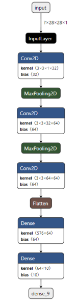
As we can see our CNN architecture has 3 convolutional layers and 2 dense layers.
Now let us train our data for 5 epochs with different optimizers.
Model Training
#Here we are compiling our model with optimizer as adam. We have a validation_split of 0.1
model.compile(optimizer='adam',loss='categorical_crossentropy',metrics=['accuracy'])
hist = model.fit(XTrain,YTrain,epochs=5,validation_split=0.1,batch_size=128)
We will train our model with different optimizers and compare the validation accuracy achieved.
| Optimizer | Validation Accuracy | |
|---|---|---|
| 0 | SGD | 96.50 |
| 1 | Adagrad | 89.28 |
| 2 | Adam | 98.97 |
| 3 | rmsprop | 98.95 |
As we can see from the table, maximum validation accuracy is achieved when we have an optimizer as adam.
Conclusion
In this article, we have discussed the various optimizers available for training deep neural networks. Further, we have experimented by training a neural network with SGD, Adam, RMSProp, and Adagrad optimizers respectively, and compared the validation accuracy. We have also seen how Adam optimizer outperformed the Adagrad and RMSprop to achieve superior performance. We also discussed in detail the variants of the gradient descent algorithm.
References
- https://arxiv.org/abs/1412.6980
- http://www.cs.toronto.edu/~tijmen/csc321/slides/lecture_slides_lec6.pdf
- https://ruder.io/optimizing-gradient-descent/index.html#adagrad
- https://arxiv.org/abs/1412.6651