Unfolding Google’s Inception Network

S.No	Lesson Title
1	Introduction
2	Problems solved by inception network
3	Inception Module
4	Inception Network Architecture
5	Conclusion

Introduction

Deep learning is a growing field with new innovations and research papers emerging frequently. Convolutional neural networks have improved a lot with new ideas to tackle frequently faced problems. One such innovative idea is the idea of inception networks. The idea of inception came out from a paper named "Going Deeper with Convolutions". The architecture proposed in this network is called GoogLeNet or Inception V1. This network put forward a phenomenal performance in the ImageNet Visual Recognition Challenge in 2014 hosted on a reputed platform for benchmarking image recognition and detection algorithms.

In this article, we'll go through the network architecture and how it helps in improving performance by tackling some commonly faced problems while training very deep networks.

Problems solved by inception network

Theoretically, the best way to improve the performance of a deep learning network is by creating bigger networks with a large number of layers of neurons in each layer. This idea of improving performance looks good but often leads to complications like overfitting due to an increase in complexity of the network and more computational power required due to an increase in the number of parameters. Another major challenge is faced when we add a new layer where we have to select a new filter size, select between convolutional or pooling layers. This can be problematic when we have a huge network and testing the addition of a new layer and tuning its hyperparameters can be time-consuming. These are some major issues that are more or less solved by the inception of the network.

The paper on the inception network mentioned before suggests the use of sparsely connected network architecture which is used in place of traditional fully connected architectures. The approach suggested allows increasing the depth of the network while not increasing the computational cost by a large amount.

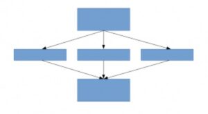
The following diagram throws some light on the basic concept of sparsely connected networks:

In the upcoming sections, we'll have a look at how this idea was implemented and what changes were made to the fully connected CNN to get an Inception Network.

Inception Module

Before jumping on to visualize the entire network we'll have a look at a smaller block of the network called the inception module. Multiple inception modules are stacked with different configurations to form an inception network.

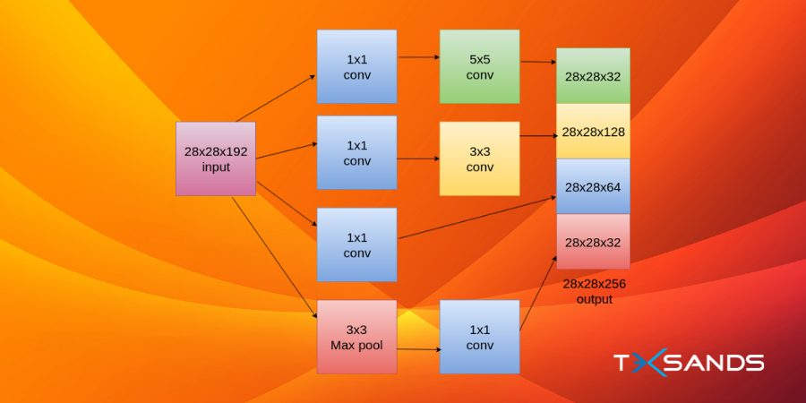
Following is an image of an inception module:

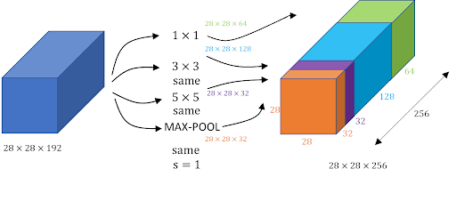
In the given figure above we have an inception block where the input is 28x28x192. Now we'll apply 1x1x64 convolution using the following rule to calculate the dimensions (this rule will be used for all the dimension related calculations):

Dimension(n2) = (n1+2p-f/s)+1

Where, n1=28 (previous layer dimension), f=1 (filter size), p = 0 (padding) , s = 1 (filter steps). Now we want a 3x3x128 convolution where we need to set the padding as 1 which basically refers to the same convolution which sets the dimension as 28x28x128 so that we can stack the outputs to get the final output. This way we can apply different filters like the max-pooling filter applied above. The only thing to keep in mind is that the width and breadth of all the outputs should be the same so that we can concatenate them at the end. In order to do this, we use padding=same for all filters except the 1×1 filter. This idea of concatenating outputs from different filters and getting a single output is at the heart of an inception network. It allows the network to learn whatever it wants.

One issue with the method we discussed above is a large number of parameters we'll get when we convolve 32 5×5 filters with 28x28x192 input volume. The final output here is 28x28x32 where we have 32 filters with 5x5x192 dimensions. Now the total number of parameters is 28x28x32x5x5x192 which is 120 million parameters which are really expensive considering this is a very small part of the entire network. In order to solve this, we can use a 1×1 convolution to reduce input dimensions. After that we can apply 5×5 convolution to get the final output:

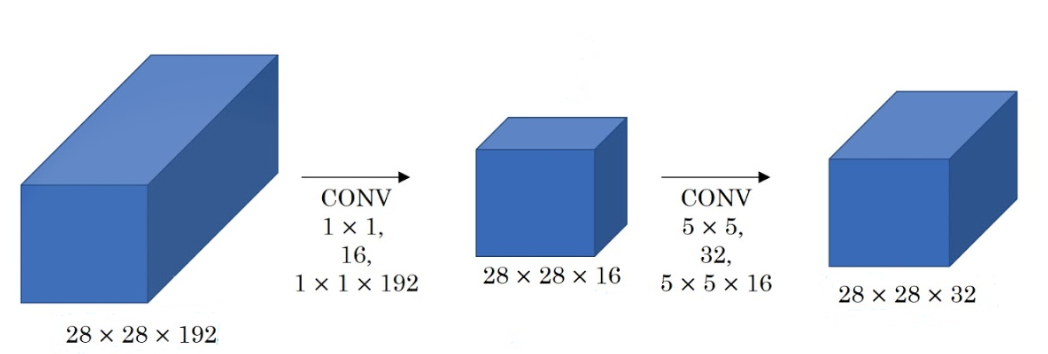
The total number of parameters in this case is 28x28x16x1x1x192 + 28x28x32x5x5x16 = 12.4 million parameters. Now, this is a significant reduction in the number of parameters compared to the 120 million parameters we got before.

This idea of using 1×1 convolutions is successful as lower-dimensional embeddings can also contain information about large patches of images. So the basic idea boils down to using a 1×1 convolution before 5×5 or 3×3 convolutions. There are other uses and interpretations of a 1×1 filter but for an inception network, we'll keep the use limited to dimensionality reduction. In the next section, we'll have a look at how this small block is embedded into a large network.

Inception Network Architecture

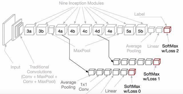
Remember the basic architecture of a traditional convolutional network where we take the output from the previous layer and feed it to the next layer and this process is repeated until the end of the network. But in an inception network, the output from the previous layer is taken and then passed on to four different layers/operations in parallel and then concatenate the output and keep repeating the process till the end. Have a look at the following figure which represents an inception network (GoogLeNet):

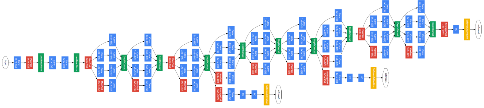
Google's inception network has 9 inception modules stacked linearly. There are 22 layers, 27 if pooling layers are counted. A global average pooling layer is added at the end of the last inception block.

One issue that inception networks face like any other deep network is vanishing gradients. In order to solve this issue, intermediate classifiers were introduced. They are represented by the yellow blocks in the above diagram. Following is a zoomed-out image of the inception network for a better understanding of these intermediate classifiers:

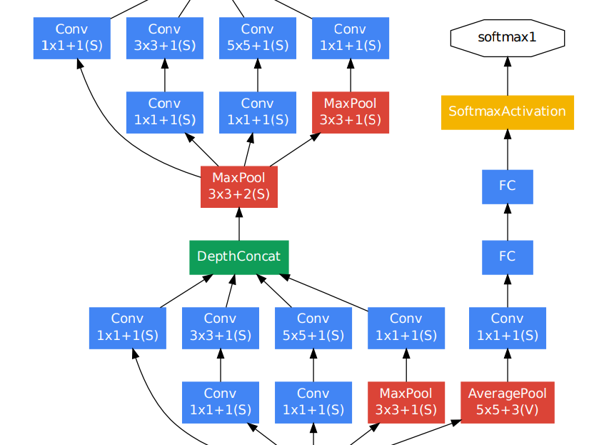
Now the final loss is a combination of intermediate loss from these classifiers and the final loss at the end. The total loss is a combination of three losses from three yellow blocks. A weight of 0.3 is given to intermediate losses. These intermediate networks stay active during the training stage and are discarded during the inference/test stage. Following is an equation for total loss:

total_loss = real_loss + 0.3 * aux_loss1+ 0.3 * aux_loss2

Have a look at the following diagram from the paper to see how the intermediate classifiers are added:

Conclusion

With this, we come to the end. Though old, the inception network produced state-of-the-art results when it was introduced in 2014 and led to more interesting research in order to get efficient architectures for deep CNN models. This research was carried on newer architectures that came into the picture which revolutionized the way deep CNN models were trained. Happy Learning!

References

1. https://www.cs.colostate.edu/~dwhite54/InceptionNetworkOverview.pdf
2. https://www.coursera.org/lecture/convolutional-neural-networks/inception-network-piR0x