Generative Adversarial Networks

S.No	Lesson Title
1	Introduction
2	Discriminative vs. Generative Modelling
2.1	The Generator Model
2.2	The Discriminator Model
2.3	GANs as a Two Player Game
3	GANs using keras
3.1	Importing and Preprocessing Dataset
3.2	Generator Model
3.3	Discriminator Model
3.4	Training
4	Conclusion

Introduction

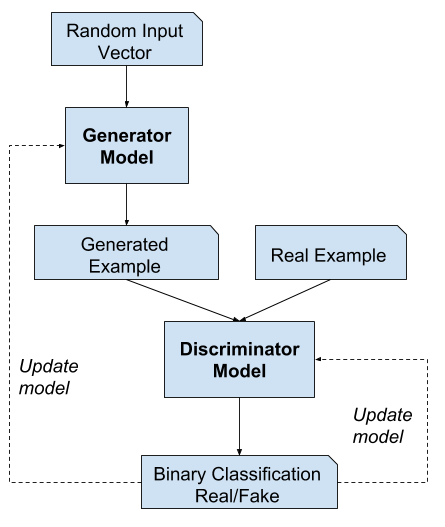
Generative Adversarial Networks which is abbreviated as GANs is a way of generative modeling using deep learning. Generative modeling is an unsupervised learning method. In this, the model automatically learns the patterns in our input data in a way that the model can be used to generate new data. GANs is a method in which we train a model by converting the problem as a supervised learning problem using two sub-models: the generator model, which we train to generate new data, and the discriminator model that tries to classify examples as either real or fake.

Discriminative vs. Generative Modelling

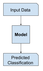
In supervised learning, one of the tasks can be to create a model which will be able to predict a class label given input variables. This kind of task is called classification.

Classification is also called discriminative modeling. We call classification as discriminative modeling because, in classification, a model has to discriminate examples of input variables across classes. A model has to make a decision as to what class the given input belongs to.

Unsupervised models which understand the distribution of input variables can be used to generate new examples in the input distribution. Hence, these models are called generative models.

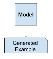
For instance, a variable may have a Gaussian distribution. In such a case, a generative model could summarize this data distribution, and then it could generate new examples which fit into the distribution of the input.

The Generator Model

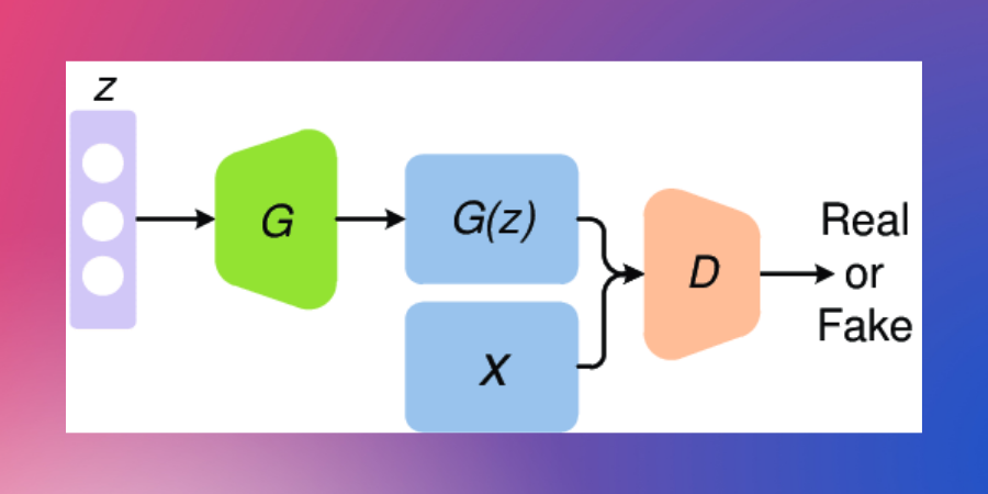
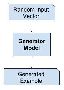
The generator model takes a random vector as input and generates a sample in the domain. The generator model takes a random vector of fixed length as input and it outputs a sample in the down. The random vector is drawn from the Gaussian distribution and it is used to seed the generative process. After training is complete, the values in the vector space will correspond to the points in the problem domain, which would form a compressed representation of the data. This vector is also called latent space. Latent variables are those variables that are important for a domain but are not directly observable.

After the training is complete, the generator model is saved and is used to generate new data.

The Discriminator Model

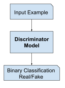
The discriminator model takes as input examples from the training dataset and the generated data. The task of the discriminator is to predict a binary class label real or fake. We fetch the real examples from the training data and the fake examples from the generator. The discriminator is a simple classification model. After the training process is complete, the discriminator is discarded as we are interested in generating new images.

GANs as a Two Player Game

The two models are trained together. The generator generates a batch of data and this batch along with the real examples from the training dataset are fed as input to the discriminator which classifies the examples as real or fake. The goal is for the generator to generate such good data that the discriminator classifies it as real.

After training on a batch of data, the weights of the discriminator are updated so that it can get better at distinguishing between real and fake data. The generator is updated on the basis of how well or how bad the generated data was able to fool the discriminator.

In this manner, the two models are competing against each other. In the sense of game theory, they are playing a zero-sum game. In this scenario, zero-sum means that if the discriminator correctly identifies real and fake data then it is rewarded, whereas the generator is penalized with large updates. On the other hand, if the generator successfully fools the discriminator, then it is rewarded and the discriminator is penalized.

GANs using Keras

Now we are going to create a GAN using keras which can generate MNIST data.

Importing and Preprocessing Dataset

First, let us import all the libraries that we need to create gans.

#Here we are importing all the libraries that we need to implement gans
from keras.datasets import mnist
from keras.layers import *
from keras.layers.advanced_activations import LeakyReLU
from keras.models import Sequential,Model
from keras.optimizers import Adam

import matplotlib.pyplot as plt
import math
import numpy as np

Now that we have imported all the files that we need, let us now import the load the MNIST dataset from keras.

#Here we are importing the MNIST dataset

(X_Train,_),(_,_) = mnist.load_data()

We have now imported our dataset. We have only imported the X_Train portion of the dataset because we will only need that to generate new images.
Let us now reshape and normalize our data.

#Here we are reshaping our dataset

print(X_Train.shape)

X_Train = X_Train.reshape((*(X_Train.shape),1))
print(X_Train.shape)

X_Train = (X_Train.astype('float32') - 127.5)/127.5

Output:

(60000, 28, 28)
(60000, 28, 28, 1)

We have now reshaped and normalized our dataset. Our dataset has 60000 images and each image is of the shape (28x28x1).

Now that we have pre-processed our dataset, let us now define some variables which we will need in this project.

NUM_EPOCHS = 50
BATCH_SIZE = 256
NO_OF_BATCHES = math.ceil(X_Train.shape[0]/float(BATCH_SIZE))
HALF_BATCH_SIZE = int(BATCH_SIZE/2)

NOISE_DIM = 100

adam = Adam(lr=2e-4,beta_1=0.5)

We have now defined all the variables that we would need for our project.

Generator Model

Now let us create the generator model.

#Here we are creating the generator model
#Upsampling 
# Start from 7 X 7 X 128
generator = Sequential()
generator.add(Dense(7*7*128,input_shape=(NOISE_DIM,)))
generator.add(Reshape((7,7,128)))
generator.add(LeakyReLU(0.2))
generator.add(BatchNormalization())

#Double the Activation Size 14 X 14 X 64
generator.add(UpSampling2D())
generator.add(Conv2D(64,kernel_size=(5,5),padding='same'))
generator.add(LeakyReLU(0.2))
generator.add(BatchNormalization())

# Double the Activation Size 28 X 28 X 1
generator.add(UpSampling2D())
generator.add(Conv2D(1, kernel_size=(5, 5), padding='same', activation='tanh'))

# Final Output (No ReLu or Batch Norm)
generator.compile(loss='binary_crossentropy', optimizer=adam)
generator.summary()

Discriminator Model

Now let us create our discriminator model.

#Discriminator - Downsampling
discriminator = Sequential()
discriminator.add(Conv2D(64,(5,5),strides=(2,2),padding='same',input_shape=(28,28,1)))
discriminator.add(LeakyReLU(0.2))

# Prefer Strided Convolutions over MaxPooling
discriminator.add(Conv2D(128,(5,5),strides=(2,2),padding='same'))
discriminator.add(LeakyReLU(0.2))


discriminator.add(Flatten())
discriminator.add(Dense(1,activation='sigmoid'))

discriminator.compile(loss='binary_crossentropy',optimizer=adam)
discriminator.summary()

Output:

_________________________________________________________________
_________________________________________________________________
Layer (type)                 Output Shape              Param #   
=================================================================
conv2d_7 (Conv2D)            (None, 14, 14, 64)        1664      
_________________________________________________________________
leaky_re_lu_7 (LeakyReLU)    (None, 14, 14, 64)        0         
_________________________________________________________________
conv2d_8 (Conv2D)            (None, 7, 7, 128)         204928    
_________________________________________________________________
leaky_re_lu_8 (LeakyReLU)    (None, 7, 7, 128)         0         
_________________________________________________________________
flatten_2 (Flatten)          (None, 6272)              0         
_________________________________________________________________
dense_4 (Dense)              (None, 1)                 6273      
=================================================================
Total params: 212,865
Trainable params: 212,865
Non-trainable params: 0
_________________________________________________________________

In the case of a discriminator, we are creating a simple CNN architecture that can predict whether an image is real or fake.

Now that we have created our discriminator, let us now create a function that will save our generated images.

#Here we are creating the functional api of our model. 
#Also we are creating a function which will generate and save our images.

discriminator.trainable = False
gan_input = Input(shape=(NOISE_DIM,))
generated_img = generator(gan_input)
gan_output = discriminator(generated_img)

#Functional API
model = Model(gan_input,gan_output)
model.compile(loss='binary_crossentropy',optimizer=adam)

def save_imgs(epoch,samples=100):
    noise = np.random.normal(0,1,size=(samples,NOISE_DIM))
    generated_imgs = generator.predict(noise)
    generated_imgs = generated_imgs.reshape(samples,28,28)
    
    plt.savefig('images/gan_output_epoch_{0}.png'.format(epoch+1))

We have now created the function to save_imgs which will save our generated images. Note that we have kept the discriminator as not trainable. This statement will be executed when the generator is training. At a time only one model will be trained. So, when the generator is being trained, the discriminator is non-trainable and vice-versa.

Training

Let us now train our models.

#Here we are training our model
for epoch in range(NUM_EPOCHS):
    epoch_d_loss = 0.
    epoch_g_loss = 0.
    
for step in range(NO_OF_BATCHES):
    #randomly select 50% real images
    idx = np.random.randint(0,X_Train.shape[0],HALF_BATCH_SIZE)
    real_imgs = X_Train[idx]
    
    # generate 50% random images
    noise = np.random.normal(0,1,size=(HALF_BATCH_SIZE,NOISE_DIM))
    fake_imgs = generator.predict(noise)
    
    
    # one sided label smoothing
    real_y = np.ones((HALF_BATCH_SIZE,1))*0.9 #Label Smoothing, Works well in practice
    fake_y = np.zeros((HALF_BATCH_SIZE,1))
    
    # train on real and fake images
    d_loss_real = discriminator.train_on_batch(real_imgs,real_y) #updates the weights of discriminator
    d_loss_fake = discriminator.train_on_batch(fake_imgs,fake_y) 
    d_loss = 0.5*d_loss_real + 0.5*d_loss_fake
    
    epoch_d_loss += d_loss
    
    
    #Train Generator (Complete Model Generator + Frozen Discriminator)
    
    noise = np.random.normal(0,1,size=(BATCH_SIZE,NOISE_DIM))
    real_y = np.ones((BATCH_SIZE,1))
    g_loss = model.train_on_batch(noise,real_y)
    epoch_g_loss += g_loss
    

if (epoch+1)%10==0:
    generator.save('models/gan_generator_{0}.h5'.format(epoch+1))
    save_imgs(epoch) 

In the above code, we are generating the HALF_BATCH_SIZE number of images, using our generator function. After that, we are training our discriminator separately on the real and the fake images. After the discriminator has been trained, we are freezing the discriminator and training our generator model.

Now that we have finished training our model, let us see the images which we have generated.

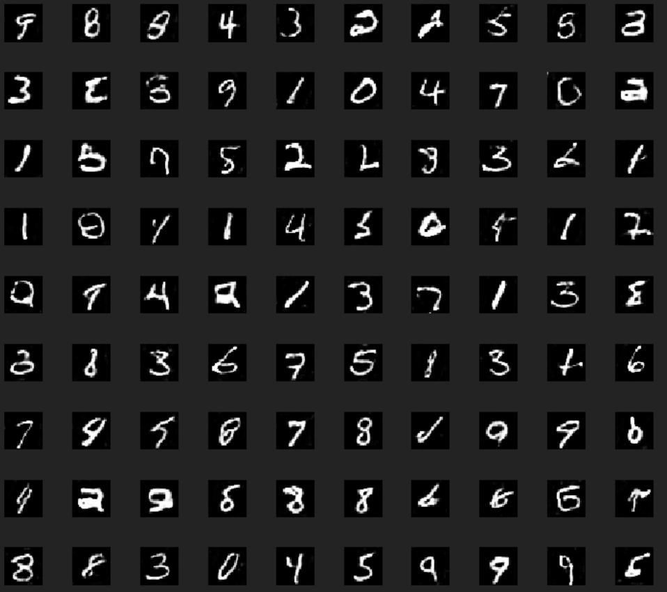
We can see that the images which we generated resemble the actual MNIST data to a great extent.

Conclusion

In this article, we have explored one more dimension of supervised learning. i.e the generative models. We have discussed in detail the Generative Adversarial Network, which involves a generator and a discriminator. We have also implemented GANs in keras on the MNIST dataset and showed the capability of the generative models.