

Exploratory Data Analysis

Course Lessons
| S.No | Lesson Title |
|---|---|
| 1 | Introduction |
| 2 | Steps in EDA |
| 2.1 | Variable Identification |
| 2.2 | Basic Data Exploration |
| 2.3 | Null Values |
| 2.4 | Outliers |
| 2.5 | Transforming Categorical Variables |
| 2.6 | Encoding |
| 2.7 | Correlation |
| 3 | Conclusion |
Introduction
Exploratory data analysis (EDA) is an approach to investigating the datasets to discover patterns, anomalies, imbalances using statistical graphics and other data visualization methods. EDA is all about making sense of the data, after which we can gather insights from it. Exploratory Data Analysis is an important step before making a machine learning model. EDA provides the context needed to develop an appropriate model - and interpret the results correctly.
Let us understand EDA in more detail by performing EDA on the wine quality dataset.
Steps in EDA
There are many steps in EDA. Some of them are as follows:
Variable Identification
In this step, we identify the predictor (input) and the target (output) variables. After this, we have to identify the category and data types of the variables.
Let us visualize the first 5 rows of our dataset.
df=pd.read_csv('winequalityN.csv')
df.head()
Output:
| type | fixed acidity | free sulphur dioxide | total sulfur dioxide | density | pH | sulphates | alcohol | quality |
|---|---|---|---|---|---|---|---|---|
| white | 7 | 45 | 170 | 1.001 | 3 | 0.45 | 8.8 | 6 |
| white | 6.3 | 14 | 132 | 0.994 | 3.3 | 0.49 | 9.5 | 6 |
| white | 8.1 | 30 | 97 | 0.9951 | 3.26 | 0.44 | 10.1 | 6 |
| white | 7.2 | 47 | 186 | 0.9956 | 3.19 | 0.4 | 9.9 | 6 |
| white | 7.2 | 47 | 186 | 0.9956 | 3.19 | 0.4 | 9.9 | 6 |
As we can see from this dataset 'quality' is our target variable and all the other variables are our predictor variables.
Basic Data Exploration
In this step, we will explore the shape and the information of the dataset. The shape of the dataset will tell us the dimensions of the dataset, like how many rows and columns we have in our dataset. info() is used to check the Information about the data and the data types of each respective attribute.
print(df.shape)
Output:
(6497,13)
As we can see, our dataset has 6497 rows and 13 columns.
Now let us gather some for information about our dataset.
print(df.info())
Output:
<class 'pandas.core.frame.DataFrame'>
RangeIndex: 6497 entries, 0 to 6496
Data columns (total 13 columns):
type                    6497 non-null object
fixed acidity           6487 non-null float64
volatile acidity        6489 non-null float64
citric acid             6494 non-null float64
residual sugar          6495 non-null float64
chlorides               6495 non-null float64
free sulfur dioxide     6497 non-null float64
total sulfur dioxide    6497 non-null float64
density                 6497 non-null float64
pH                      6488 non-null float64
sulphates               6493 non-null float64
alcohol                 6497 non-null float64
quality                 6497 non-null int64
dtypes: float64(11), int64(1), object(1)
memory usage: 660.0+ KB
None
We can see from the output that the 'type' attribute has characters instead of numbers as it is of the type object. The data types in our entire dataset are float64(11), int64(1), and object(1). Now we will gather some more insights into our dataset using the 'describe' method. This will tell us the mean, median, mode, maximum value, minimum value, etc. of each column.
| fixed acidity | volatile acidity | citric acid | residual sugar | chlorides | |
|---|---|---|---|---|---|
| count | 6487 | 6489 | 6494 | 6495 | 6495 |
| mean | 7.216579 | 0.339691 | 0.318722 | 5.444326 | 0.056042 |
| std | 1.29675 | 0.164649 | 0.145265 | 4.758125 | 0.035036 |
| min | 3.8 | 0.08 | 0 | 0.6 | 0.009 |
| 25% | 6.4 | 0.23 | 0.25 | 1.8 | 0.038 |
| 50% | 7 | 0.29 | 0.31 | 3 | 0.047 |
| 75% | 7.7 | 0.4 | 0.39 | 8.1 | 0.065 |
| max | 15.9 | 1.58 | 1.66 | 65.8 | 0.611 |
Here we can see the count, mean, standard deviation, minimum value, maximum value of each of the columns in our dataset.
Null Values
The next step in EDA is to check and remove null values in our dataset. If there are null values then we won't be able to apply machine learning algorithms to our dataset, so it is imperative that we eliminate them.
df.isnull().sum()
Output:
type                     0
fixed acidity            10
volatile acidity         8
citric acid              3
residual sugar           2
chlorides                2
free sulfur dioxide      0
total sulfur dioxide     0
density                  0
pH                       9
sulphates                4
alcohol                  0
quality                  0
dtype: int64
Here we can see that the attributes, 'fixed acidity', 'volatile acidity', 'citric acidity', 'residual sugar', 'chlorides', 'pH' and 'sulphates' all have missing values. We need to remove them.
The ways to handle null values are as follows:
- We can drop the missing values. This can be done when the number of missing values is less.
- For numerical columns, we can replace the missing values with the mean values of the column.
- For numerical columns, we can replace the missing values with the median of the column.
- For categorical columns, we can replace the missing values with the mode of the column.
Since all the columns which have null values are numeric, so we can replace the null values in them with their means.
#Here we are replacing all the null values in a column with the mean of that particular column.

df['fixed acidity'].replace(np.nan,df['fixed acidity'].mean(),inplace=True)
df['volatile acidity'].replace(np.nan,df['volatile acidity'].mean(),inplace=True)
df['citric acid'].replace(np.nan,df['citric acid'].mean(),inplace=True)
df['residual sugar'].replace(np.nan,df['residual sugar'].mean(),inplace=True)
df['chlorides'].replace(np.nan,df['chlorides'].mean(),inplace=True)
df['pH'].replace(np.nan,df['pH'].mean(),inplace=True)
df['sulphates'].replace(np.nan,df['sulphates'].mean(),inplace=True)
df.isnull().sum()
Output:
type                    0
fixed acidity           0
volatile acidity        0
citric acid             0
residual sugar          0
chlorides               0
free sulfur dioxide     0
total sulfur dioxide    0
density                 0
pH                      0
sulphates               0
alcohol                 0
quality                 0
dtype: int64
As we can see, now our dataset does not have any missing values.
Outliers
Our next step is to detecting and treating outliers. Outlier is an observation that appears far away and diverges from an overall pattern in a sample. Let us see the outliers in the column 'fixed acidity'.
#boxplot will help us see the outliers in a particular column
df.boxplot(column=["fixed acidity"])
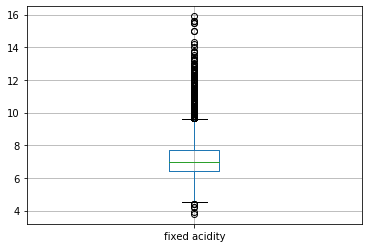
The black dots represent the outliers in our column.
We can remove outliers by either dropping the outliers or by replacing the outlier values using IQR.
def remove_outlier(col):
    sorted(col)
    Q1,Q3= col.quantile([0.25,0.75])
    IQR=Q3-Q1
    lower_range= Q1-(1.5* IQR)
    upper_range= Q3+(1.5*IQR)
    return lower_range,upper_range
low,high=remove_outlier(df["fixed acidity"])
df["fixed acidity"]=np.where(df["fixed acidity"]>high,high,df["fixed acidity"])
df["fixed acidity"]=np.where(df["fixed acidity"]<low,low,df["fixed acidity"])
Here, by using IQR we have removed outliers of the column 'fixed acidity'. Similarly, we can remove outliers of all the columns. Let us see the boxplot of the column 'fixed acidity' again in order to see whether or not the outliers have been removed.
df.boxplot(column=["fixed acidity"])
Output:
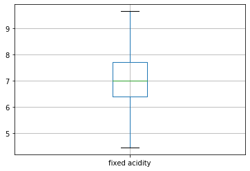
As we can see, now we don't have any outliers.
Transforming categorical variables
The column 'type' is a categorical variable as it has only two categories, white and red. Our machine learning algorithm will not be able to understand string inputs, so we will have to convert our text data to an integer. This will be achieved through the LabelEncoder library inside Sklearn.
from sklearn.preprocessing import LabelEncoder
label=LabelEncoder()

#Here we are transforming our categorical data

df['type']=label.fit_transform(df['type'])
Now our column 'type' has integers instead of characters.
Encoding
One hot encoding is used to create dummy variables so that we can replace the categories in a categorical variable into features of each category and we can represent each feature using 1 or 0 based on whether or not the categorical value is present or absent in the record.
Correlation
Correlation helps us to understand how all the variables are related to one another. It helps us see how important a particular feature is and whether or not we have any multicollinearity.
import seaborn as sns

#Here we are computing the correlation of our variables.
corr = df.corr()
plt.subplots(figsize=(30,10))

#We are now plotting our correlation matrix using heatmap in seaborn
sns.heatmap( corr, square=True, annot=True,fmt=".1f")
Output:
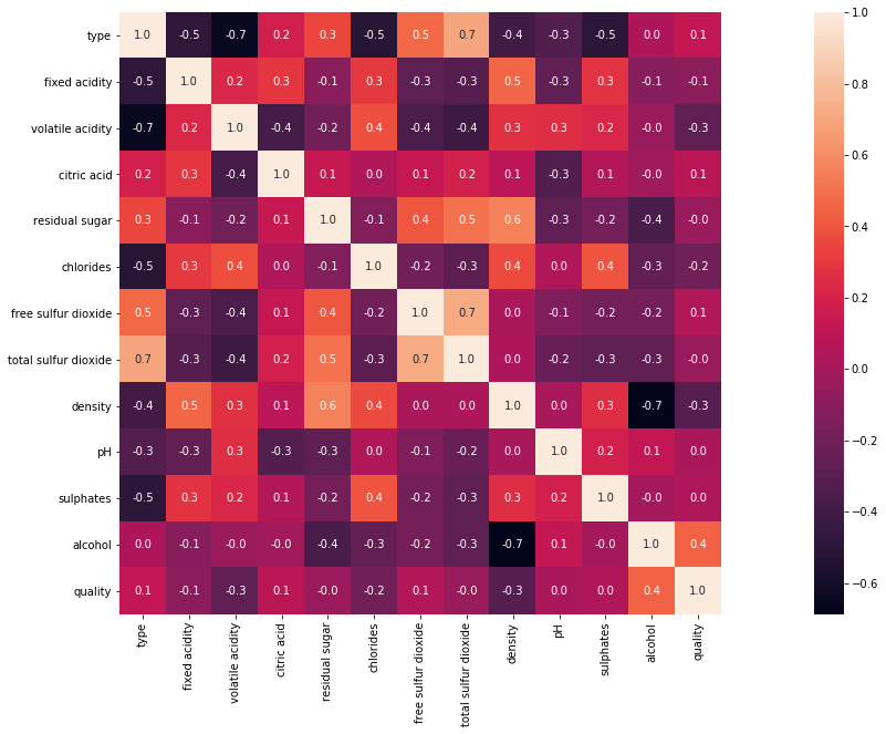
The blocks that are shaded lighter mean that they have a higher degree of relation.
After this we can Standardize our data, we can visualize it using matplotlib, seaborn, or any other visualization libraries available in python so that we can get more information regarding our data and we can perform feature engineering.
Conclusion
In this article, we have explored Exploratory Data Analysis in machine learning. Also, we have discussed various steps involved in EDA, such as removing null values, one-hot encoding, etc. Further, we have seen how to perform EDA in python. Hope this tutorial will help in exploiting EDA in real-time data. Happy learning.
References
- https://medium.com/swlh/exploratory-data-analysis-what-is-it-and-why-is-it-so-important-part-1-2-240d58a89695
- https://www.upgrad.com/blog/exploratory-data-analysis-and-its-importance-to-your-business/#:~:text=Exploratory%20Data%20Analysis%20is%20a,and%20interpret%20the%20results%20correctly
- https://towardsdatascience.com/ways-to-detect-and-remove-the-outliers-404d16608dba