Comparison of Classification Algorithms

S.No	Lesson Title
1	Introduction
1.1	Applications of Classification
2	Types of Classifiers
2.1	Naive Bayes Classifier
2.2	Support Vector Machine
2.3	K-Nearest Neighbours (KNN)
2.4	Decision Tree
2.5	Random Forest
3	Performance
3.1	Preprocessing
3.2	Calculating Performance of Different Classifiers
4	Conclusion

Introduction

Classification is an essential ability of human beings involving recognizing the shared features or the similarities between the elements. The research community is trying its level best to introduce various classification algorithms to solve a day-to-day challenging classification problem. In this article, we will introduce and compare some of the prominent classification algorithms.

Applications of Classification

• speech recognition
• handwriting recognition and so on.

Types of Classifiers

Binary Classifiers : Classification with just 2 different classes. For eg: Male and Female, Spam and Non-spam mail, Positive and Negative sentiment, etc.

Multi-Class classifiers : Classification involving more than two classes. For eg: Types of soil, Types of music, etc.

Here we will look at 5 different classifiers. We will also see their performance on the digits dataset from sklearn. The classifiers we will see are, K-Nearest Neighbours, Naive Bayes, Random Forest, Decision Trees and Support Vector Machines.

Naive Bayes Classifier

Naive Bayes is a probabilistic classifier which was inspired by the Bayes hypothesis. Under a straightforward suspicion which is the properties are restrictively free.

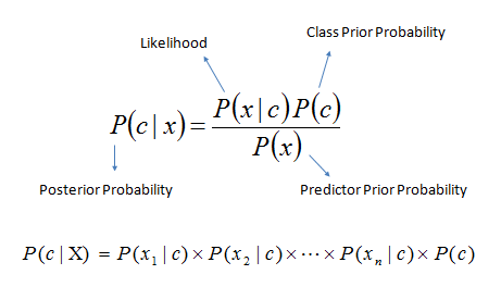
The classification is led by deriving the maximum posterior which is the maximal P(Ci|X) with the above assumption applying to Bayes hypothesis. This assumption enormously diminishes the computational expense by just tallying the class dissemination. Even though the assumption is not valid in most cases as the features are dependent, Naive Bayes is able to perform very well. It is a simple algorithm to implement. It can be scaled to be applied on large datasets since it takes linear time.

Naive Bayes tends to suffer from a problem called the zero probability problem. This occurs when the conditional probability is zero for a particular feature. In such cases, the classifier is not able to give a valid prediction. This can be fixed using a Laplacian estimator.

Advantages: Naive Bayes classifier requires small amount of training data and it is extremely fast as compared to more complex classifiers.

Disadvantages: Naive Bayes is not a good estimator.

Support Vector Machine

Support Vector Machine (SVM) is a supervised machine learning algorithm which can be used for both classification or regression challenges. However, it is mostly used in classification problems. In the SVM algorithm, we plot each data item as a point in n-dimensional space (where n is number of features we have) with the value of each feature being the value of a particular coordinate. Then, we perform classification by finding the hyper-plane that differentiates the two classes very well.

Advantages: SVM is good for both linearly and nonlinearly separable data. It is effective in high dimensional spaces and it is also memory efficient.

Disadvantages: SVM does not provide probability estimates directly. They are calculated using five-fold-cross validation.

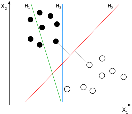
In the above diagram, H1 is not a good hyperplane as it does not separate the classes. H2 separates both the classes but it has a small margin. H3 is the maximum margin hyperplane.

Parameters of SVM: There are 3 main parameters which we could tune while constructing a SVM classifier. They are: Type of kerner, Gamma value and C value.

K-Nearest Neighbours(KNN)

KNN classifies an object by taking a majority vote of the object's neighbours. The object is then assigned to the class which is most common among its k nearest neighbour, where k is the integer explicitly defined.

KNN is a non-parametric, lazy algorithm. It is non-parametric because it does not make any assumption on data distribution (which means that the data does not have to be normally distributed). It is lazy because it does not learn any model and make generalization of the data, meaning it does not train on any data.

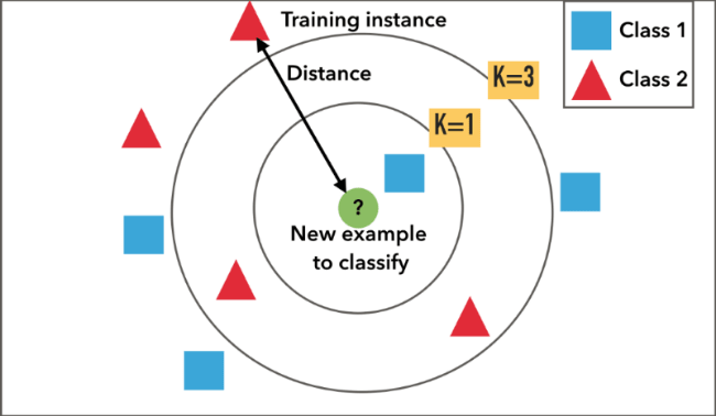
Our query point is classified by taking a majority vote of the K nearest neighbours of each point.

Advantages: KNN is easy to implement, it is can handle noise in data, and it is effective if the data is large.

Disadvantages: We need to determine the optimum value of K and that is computationally expensive.

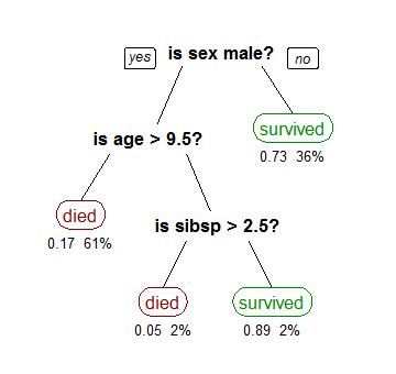
Decision Tree

Decision Tree, makes decisions using a tree-like model. It splits our dataset into two or more homogeneous sets (or leaves) based on the most significant differentiators in your input variables. In order to pick a differentiator, the decision tree considers all features and does a binary split on them. It will then pick the one with the least cost (i.e. highest accuracy), and repeats recursively, until it successfully splits the data in all leaves (or reaches the maximum depth).

Advantages: Decision Tree is easy to understand and visualise, it requires less data preparation, and it can handle both numerical and categorical data.

Disadvantages: Decision tree can become complex trees which do not generalise well, and they can be unstable as small variations in the data might result in a completely different tree being generated.

Random Forest

Random forest is an ensemble model which creates multiple trees and classifies objects based on the "votes" of all the trees. i.e. An object is assigned to a class which has most votes from all the trees. This helps to reduce the problem of overfitting.

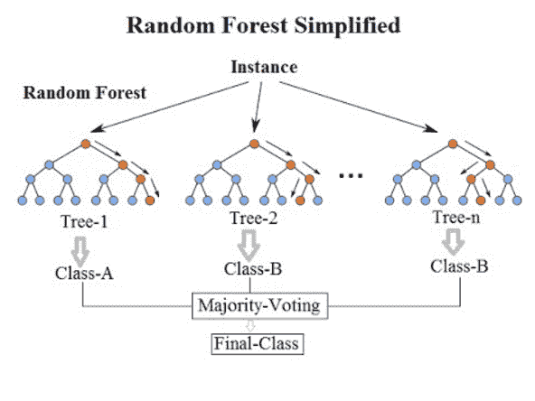
Random forest classifier fits a certain number of decision trees on various samples of datasets and computes their average to improve the predictive accuracy of the model and controls over-fitting. The sub-sample size is always the same as the original input sample size but the samples are drawn with replacement.

Advantages: Random forest classifier is more accurate than decision trees in most cases and it reduces overfitting.

Disadvantages: It has slow prediction time.

Performance

Now let us look at how these classifiers perform. We will use the digits dataset in sklearn and we are going to train each classifier on that data. After that we will compute the performance of each classifier.

#Here we have imported all the libraries required for our analysis
import numpy as np
import pandas as pd
import matplotlib.pyplot as plt
from sklearn.datasets import load_digits

We have imported all the basic libraries that we need for our analysis. Our next step is to import the dataset.

Preprocessing

digits = load_digits()
X = digits.data
Y = digits.target
print(X.shape)
print(Y.shape)
from sklearn.model_selection import train_test_split

X_train, X_test, y_train, y_test = train_test_split(X, Y, test_size=0.5, random_state=0)

Output:

(1797, 64)
(1797,64)

As we can see we have 1797 samples in our dataset. Each sample has 64 features. We will now visualize one of the samples.

plt.imshow(X[1].reshape(8,8),cmap='gray')
plt.show()
print(Y[1])

Output:

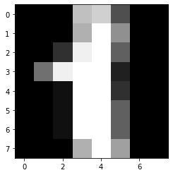
As we can see the image is of the digit 1.

Calculating Performance of Different Classifiers

We will now train each model on this dataset.

#Here we are importing KNN classifier from  sklearn and we are training the model on our dataset. Finally we are outputting the score that our model achieved on the test datset.
from sklearn.neighbors import KNeighborsClassifier
neigh = KNeighborsClassifier()
neigh.fit(X_train,y_train)
neigh.score(X_test,y_test)

Output:

 0.9777530589543938

As we can see, the KNN classifier got an accuracy of 97.75%.

Now we will create a Naive Bayes classifier.

#Here we are importing Gaussian Naive Bayes classifier from  sklearn and we are training the model on our dataset. Finally we are outputting the score that our model achieved on the test datset.

from sklearn.naive_bayes import GaussianNB
gnb = GaussianNB()
gnb.fit(X_train,y_train)
gnb.score(X_test,y_test)

Output:

0.8342602892102335

As we can see, the Naive Bayes classifier got an accuracy of 83.42%.

#Here we are importing Decision Tree classifier from  sklearn and we are training the model on our dataset. Finally we are outputting the score that our model achieved on the test datset.

from sklearn.tree import DecisionTreeClassifier
clf = DecisionTreeClassifier()
clf.fit(X_train,y_train)
clf.score(X_test,y_test)

Output:

 0.8331479421579533

As we can see, the Decision Tree classifier got an accuracy of 83.31%.

#Here we are importing Random Forest classifier from  sklearn and we are training the model on our dataset. Finally we are outputting the score that our model achieved on the test datset.

        from sklearn.ensemble import RandomForestClassifier
clf = RandomForestClassifier()
clf.fit(X_train, y_train)
clf.score(X_test,y_test)

Output:

 0.967741935483871

As we can see, the Random Forest classifier got an accuracy of 96.77%.

#Here we are importing SVM classifier from  sklearn and we are training the model on our dataset. Finally we are outputting the score that our model achieved on the test datset.

from sklearn.svm import SVC
clf =SVC()
clf.fit(X_train, y_train)
clf.score(X_test,y_test)

Output:

 0.9877641824249166

As we can see, the SVM classifier got an accuracy of 98.77%.

Conclusion

We have now seen the performance of all the classifiers that we have discussed and we can clearly see that the SVM classifier has the highest accuracy. It is important to note here that we have used the base model of each classifier. We have not performed any hyperparameter tuning. There is a chance that the performance of each classifier will change after performing hyperparameter tuning.