

Autoencoders
Course Lessons
| S.No | Lesson Title |
|---|---|
| 1 | Introduction |
| 2 | What are Autoencoders? |
| 3 |
Autoencoders vs PCA |
| 4 |
Types of Autoencoders |
| 5 | Conclusion |
Introduction
The field of deep learning has gained a lot of attraction in the last few years. The most popular problems that are solved by deep learning models tend to use supervised deep learning models. For example, problems related to image recognition, speech recognition, sentiment classification are traditionally a part of supervised deep learning. The unsupervised models for deep learning are not commonly used or discussed like their counterparts (supervised models). There are many popular unsupervised models such as self-organizing maps (SOM), autoencoders, Deep Boltzmann machines (DBM) etc. In this article we'll keep our focus on autoencoders which have gained popularity in the last few years.
Autoencoders have played a crucial role in solving many problems in the last few years such as data anomaly detection, data denoising, information retrieval, etc. They have also helped in overcoming the shortcomings of many traditional dimensionality reduction techniques such as PCA, SVD. Let's get started. In this article, we'll try to shed some light on the unsupervised side of deep learning models, specifically autoencoders. We'll aim at an exhaustive yet simple explanation of autoencoders.
What are Autoencoders?
As discussed before autoencoders are unsupervised deep learning models that are used primarily for dimensionality reduction. The basic idea is to map input data to output data and learn the encodings in the process. We also introduce a bottleneck in our model architecture which forces the model to learn a compressed knowledge representation of the original input. Following is a quote from Francois Chollet (Machine Learning Researcher at Google) from Keras Blog:
"Autoencoding" is a data compression algorithm where the compression and decompression functions are 1) data-specific, 2) lossy, and 3) learned automatically from examples rather than engineered by a human.
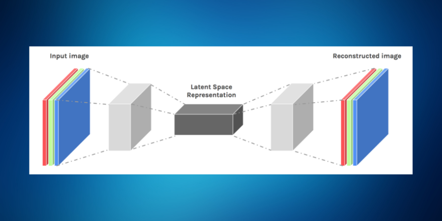
Have a look at the following image to get a preliminary idea of the basic working of an autoencoder:
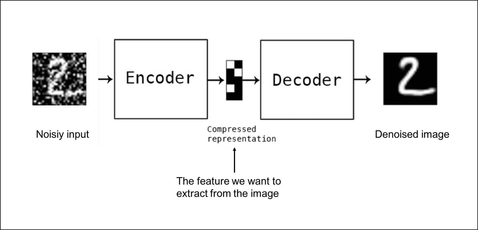
Now from the image, you can see that an autoencoder comprises two important components, encoder, and decoder. Let's see how these individual components work.
The job of the encoder is to take the input and encode it. The input is in the form of a vector. Now if the input vector is x then let the encoded function be f(x). Now the most important part comes. Autoencoders have hidden layer (or hidden layers) that learn the encodings from the data and decode it. These hidden layers are responsible for data compression, encoding/decoding i.e. in simpler terms these layers form the heart of an autoencoder. The encoding function is learned by encoder hidden layers. The hidden layer in the middle of the encoder and decoder hidden layers learns the input encodings that are encoded by the encoder i.e. h=f(x). Have a look at the following image (first two layers form encoder, the middle layer is bottleneck hidden layer or the layer that contains encoded data, final two layers form the decoder):
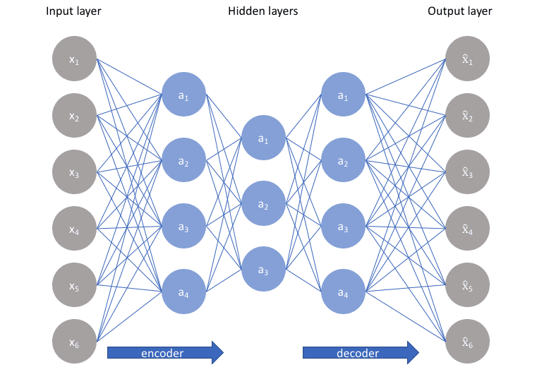
Sometimes the hidden layer in the middle is also considered a part of both encoder and decoder. It's called the bottleneck hidden layer. After the encodings are learnt by encoder hidden layers, the decoder hidden layers or the decoder function tries to reconstruct input data. If we define the decoder function as g then the reconstruction is r = g(f(x)). This is how autoencoders work in very simple terms.
The next step is to evaluate and train the network by minimizing the reconstruction error L(x,r). The reconstruction error measures the difference between the reconstructed output r and original input x. One more thing to observe is the bottleneck type structure when you move from the encoder to decoder layers. This stops the model from simply memorizing the input values by passing these values through the network. Have a look at the figure given below:
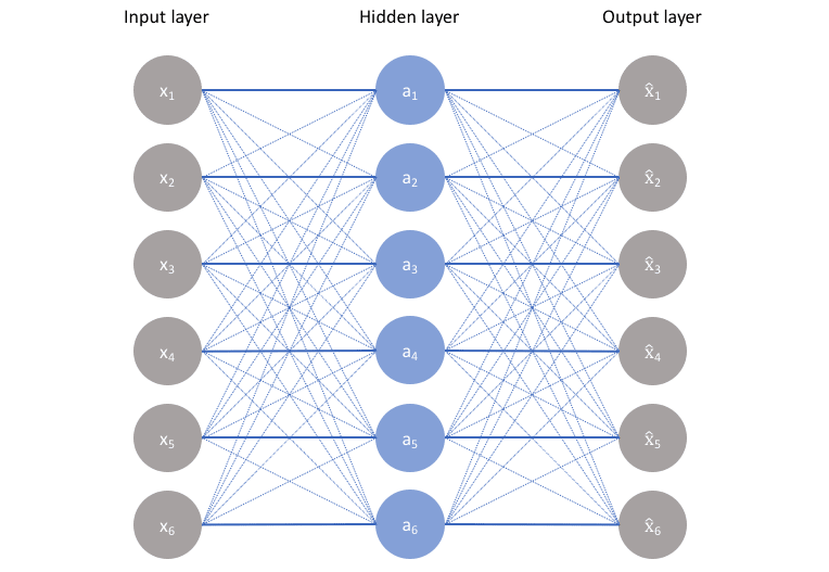
In the figure above without any bottleneck, the network will memorize the inputs and pass them through the network. Now there is a tradeoff considering what we have said. On one hand, we want our model to learn efficient encodings which can be later decoded to get a representation of data close to the input, and on the other hand, we don't want the model to blindly memorize everything i.e. we need to make sure the model is neither too good nor too bad. If you are building an ideal autoencoder it should balance the following two things:
- It should be sensitive enough to accurately encode the data and build reconstruction with the least error.
- It should be insensitive enough to make sure the network doesn't overfit the training data or simply memorize it in the worst case.
In simpler words we want the model to retain only those variations in data that are required to reconstruct the input and drop other redundancies within the input. This can be done by introducing a loss function where one term pushes our model to be more sensitive to input i.e. learn more and the other terms discourage overfitting/memorization (i.e. add regularizer to a standard loss function).
The next question that comes in our mind is the usage of autoencoders for dimensionality reduction when we already have other algorithms like PCA. We'll discuss this in the upcoming section.
Autoencoders vs PCA
PCA is the first thing that pops up in our minds when we talk about dimensionality reduction. This happens because of its widespread popularity. Both PCA and Autoencoders transform data to lower-dimensional representation by learning important features from the input data which also reduces the reconstruction cost from lower to higher dimensions. Now when we see how PCA transforms data to a lower dimension we realize that PCA does linear projections of data to lower dimensions which are orthogonal. The idea is to preserve the variance that was there in higher dimensions. Where is the problem in such a transformation?
The main problem arises due to the fact that PCA does a linear transformation. This means that any relation or important input information that is non-linear is lost. This problem is resolved in autoencoders when we use non-linear activation functions in our hidden layers. These activation functions are capable of learning input properties that are non-linear. One interesting fact is that if we use linear activation function for autoencoders we would observe a dimensionality reduction similar to the one observed for PCA.
Types of Autoencoders
There are different types of architectures for an autoencoder and in these sections, we'll discuss a few of them. Let's get started.
1. Undercomplete Autoencoder - This is the simplest architecture where the basic idea is to reduce the number of nodes in the hidden layer to constrain the amount of information that flows through the network. If we use this idea combined with penalties for wrong reconstructions then our model tries to learn the best possible features from the input which are most helpful while decoding back from the "encoded" state. The following figure represents the model architecture we are talking about:

This network can be thought of as a more powerful nonlinear generalization of PCA as neural networks are capable of learning nonlinear relationships. These autoencoders are capable of learning non-linear surfaces in higher dimensions whereas PCA attempts to find a lower-dimensional hyperplane to describe original data.
There is no regularization term in loss functions of under complete autoencoders which leaves us with carefully setting the number of nodes in hidden layers to minimize the reconstruction error. For deep autoencoders with multiple hidden layers, we have to be careful with the capacity of the encoder and decoder layers. Even if the bottleneck layer is one hidden node our model can still memorize the training data by learning some arbitrary function to map data to some index.
In order to take care of the memorizing power of autoencoders, we apply some techniques for the regularization of networks in order to encourage generalization for unseen data. Some of the techniques are mentioned below in the form of different architectures.
2. Sparse Autoencoders - This is an alternative method where we are not required to reduce the number of nodes in the hidden layer to introduce an information bottleneck. Instead, we use a loss function that penalizes activations within a layer. In simpler words, we'll try to make sure that our model learns encodings and decodings which rely on a small number of active neurons. This is similar to the dropout regularization we see in many other neural network architectures.
Following is a figure showing a sparse encoder where opaque nodes correspond to the activated nodes. The activation of a node depends on the input i.e. for different inputs different nodes can get activated based on the information that input carries.
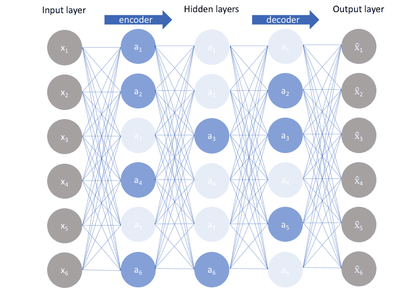
By using this method different nodes learn different information and get activated only when the input carries that specific information. This helps in reducing the network's capacity to memorize the data but also makes sure the network can learn to extract important features from the data.
There are two different methods using which we can impose the sparsity constraint. They involve adding some term to loss function to penalize excessive activations by measuring them. Following are the two activation methods:
- L1 Regularization - Here we add a term to our loss function which is basically the activation vector for a hidden layer. Vector a for activation in layer h for observation i, with scaling parameter λ is added.
-
KL-Divergence - The main idea behind KL divergence is to measure the difference between two distributions. In order to use KL-Divergence, we define a sparsity parameter that denotes the average activation of neurons over a large number of observations. This parameter is calculated as
ρ̂j =
1 mΣaih(x) where j refers to a specific neuron in layer h, an average of activation of m training examples are taken where each individual training example is denoted as x. When we try to put a constraint over the average value of neuron activations over a large number of samples we force them to fire a few times so that the average value stays low to reduce the loss. The distribution of parameter ρj an be assumed to have a Bernoulli distribution so that we can use KL divergence to compare the ideal distribution ρj and the observed distribution ρ̂j
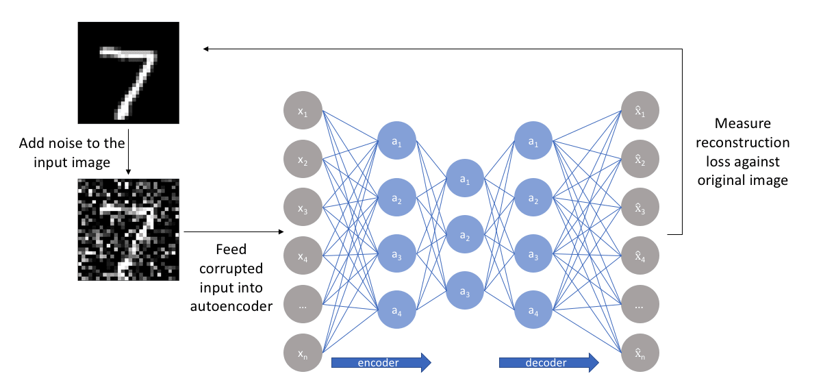
- Denoising Autoencoders - This approach uses the idea of changing the input and output we feed to our autoencoder. In simpler terms, we add some noise to our inputs but we keep the noiseless data as our outputs. This approach makes sure our model is not able to develop a mapping to simply memorize the training data because input and output are not the same. Instead, our model learns to map the input data to lower dimensions such that the data in lower dimensions accurately describes the input data without noise or the output data. If this happens then our model has learned to cancel out the noise without memorizing the input data. Following is a figure of how the architecture looks:
L(x,x̂ )+ λ ∑|aih|
L(x,x̂ )+ ∑i KL (ρj || ρ̂ j)
We'll not go deeper into the math of KL-Divergence but the final equation is a simple one that can be easily used for calculations of divergence between two Bernoulli distributions.
Conclusion
We have learned that autoencoders are models that are capable of finding structure within data with which they can develop a compressed representation of data. Many variants of the simple autoencoder are there which work on the basic idea of not letting the architecture memorize it all but at the same time allowing it to learn important features of the input data. You can even think of your own way to implement this idea! Happy Learning!